Post-Training & Alignment
Turning a pre-trained model into one that does what we want.
9 papers
Written by Junkun Yuan.
Click here to go back to main contents.
Table of contents ▶
Papers are displayed in reverse chronological order. High-impact or inspiring works are highlighted in red.
Preference Optimization
Finite Difference Flow Optimization for RL Post-Training of Text-to-Image Models
UC Berkeley · NVIDIA
arXiv, 2026
Mar 13, 2026 FDFO (4) code (117)
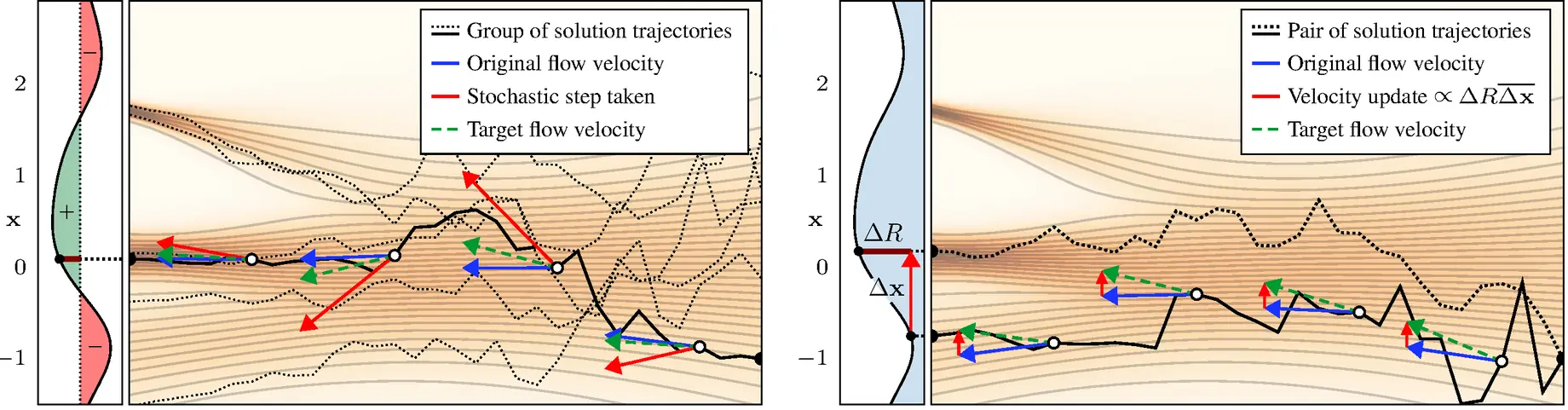
A pair of trajectories from one noise, every step bent toward the reward-weighted image difference — the whole sampling run as one action.
-
Why per-step updates are mostly noise (§1, §3.2). In an MDP each stochastic step is an action reinforced by the trajectory's advantage: a small part of every update helps the reward, the rest drifts what no reward watches — styles cycle, grid artifacts appear past ~500 epochs.
-
The whole run is one action (§4). Rollouts , from one noise with mild stochasticity; , , and the velocities at all steps of both bend toward , which points from the worse image to the better — no step credited for its own noise.
-
Why an endpoint direction works mid-trajectory (§4.1, App. C.4). The update needs , the Jacobian of the flow from step ; it holds in expectation if is positive semi-definite — exact for optimal transport, which diffusion flows approximate, SDEdit's bet too.
-
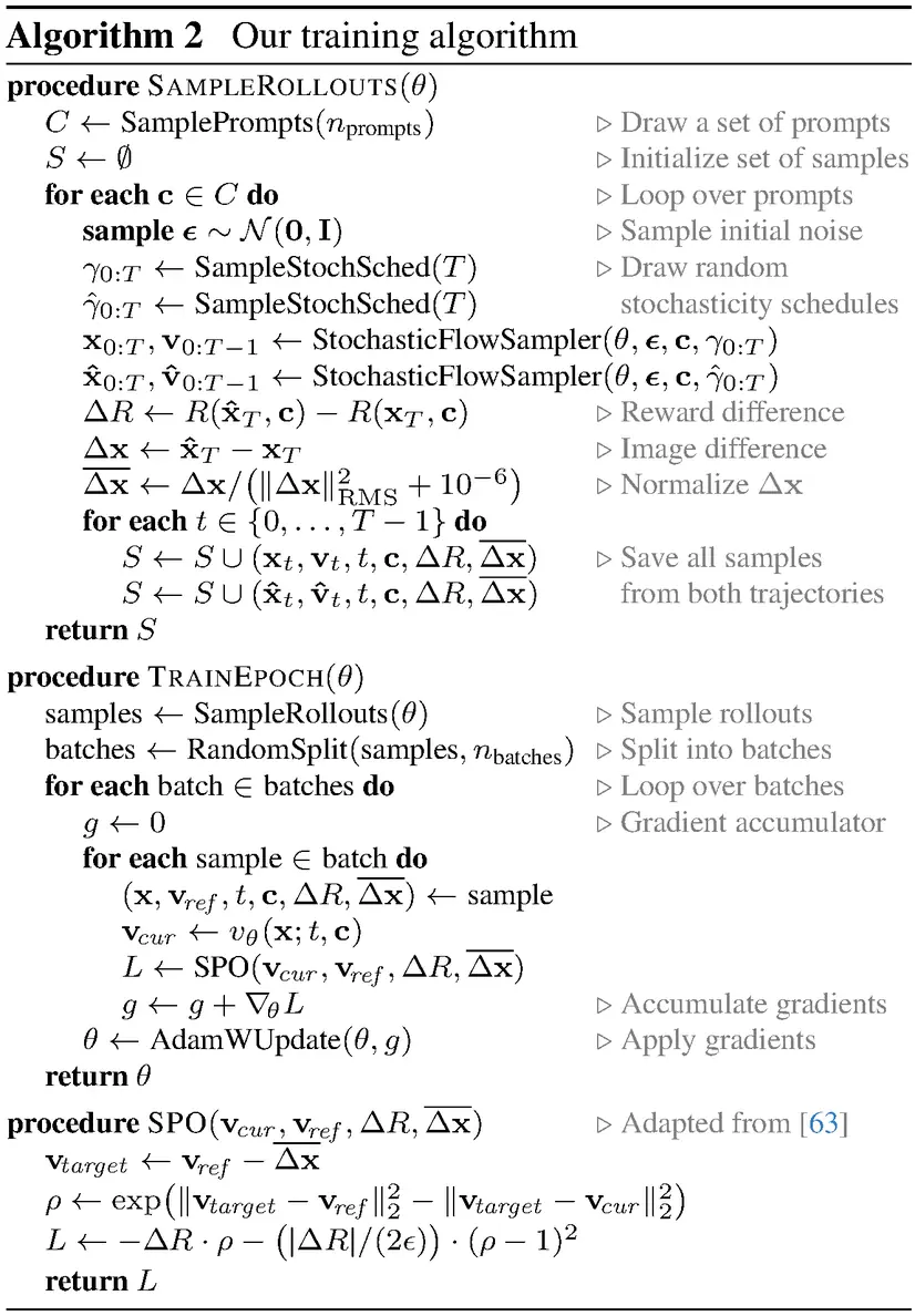
A stochastic sampler that stays on schedule (Alg. 1, B.1). Overshoot the Euler step to lower noise, then add fresh noise back to — EDM's trick, so the network's time stays right; , the noise fraction re-drawn, is 0.0025 everywhere. Flow-GRPO alone: 71.06 → 76.74 (Fig. 8 B):
-
Normalize the difference (§4.3). is, to first order, proportional to , so counts the pair's distance twice; the signal used is , the difference over its own mean square. Without it 82.13 → 79.74 and training turns unstable (Fig. 8, H).
-
Clipping without a likelihood (Alg. 2). With no likelihood for PPO's ratio, each stored velocity gets the target and a proxy ratio from two regressions; SPO then penalizes straying far from the rollout's velocity, . PPO ties (G, 81.99) only under the interval schedule:
-
Batching, and what is switched off (§4.3, Tab. 1). 432 prompt pairs per epoch at , 34,560 stored samples, 4 batches, Flow-GRPO's memory; LoRA rank 32 on SD3.5-M; EMA off (strictly harmful), KL and CFG off, so the algorithms and not the regularizers are compared.
-
Uniform stochasticity wins (B.2, Fig. 20). Against constant (U), an interval schedule perturbs one random window (I), a prior schedule only the seed (P), with optional gradient weighting: U 82.13 / 84.25 at 200 epochs / best, I 82.29 / 83.50 yet weighting-sensitive, P 70.79 / 80.51.
-
Finite differences are a smoothed gradient (App. C). Perturb the step- image, , finish both ODEs, form . With the flow from , its Jacobian, Taylor and Stein's lemma make its expectation a smoothed gradient:
- What the identity buys (App. C.3–C.5). backpropagates the gradient of a reward smoothed by a Gaussian of covariance — discontinuity smoothed away — the extra distorts it, and §4.1's condition is a quadratic form in a near-positive-definite matrix, so it ascends:
# fdfo/sampling.py: EDM churn on a flow (Alg. 1, Eq. 4-5).
r = s / (1 + gamma - gamma * s)  # overshoot past s
x_over = x + (r - t) * v  # Euler step to r
noise = r * sqrt((1 + gamma)**2 - 1) * randn_like(x)
x = (x_over + noise) / (gamma * r + 1)
# The seed is churned as well, x0 = (eps + noise0)/(gamma+1):
# the pair never shares its noise exactly; gamma = 0.0025.

# fdfo/rewards.py: the VLM reward is one next-token contrast.
r_vlm = sigmoid(logits[yes] - logits[no])  # x100 in the paper
r = r_pick + 0.1 * r_vlm  # the "combined" preset

# fdfo/train_loop.py: branches are interleaved rows; each is
# pushed toward the better image with its own sign, halved.
dR = stack((r1 - r2, r2 - r1), 1).reshape(-1) / 2
dx = stack((x1 - x2, x2 - x1), 1).reshape(-1, *shape) / 2
dx = dx / (dx.pow(2).mean(dims, keepdim=True) + 1e-6)

v = lora_transformer(x_t, t, c)  # v_cur, guidance_scale = 1
v_target = (v_ref - dx).detach()  # dt < 0: -dx moves x by +dx
ps = -((v - v_target) ** 2).mean(dims)  # means, not sums
ps_ref = -(dx ** 2).mean(dims)  # the same loss at v = v_ref
ratio = exp(ps - ps_ref)  # SPO's proxy likelihood ratio
loss = -dR * ratio + dR.abs() / (2 * 0.03) * (ratio - 1)**2
if kl_weight > 0:  # 0 in every configuration used
    loss = loss + kl_weight * ((v - v_base) ** 2).mean()
clipfrac = ((ratio - 1).abs() > 0.03).float().mean()  # logged

# 432 pairs x 2 x 40 steps per epoch, shuffled across ranks
# into 4 AdamW steps of 8,640; lr 3e-5, grad clip 1, no EMA.
# LoRA r = 32, alpha 64, on the attention projections only.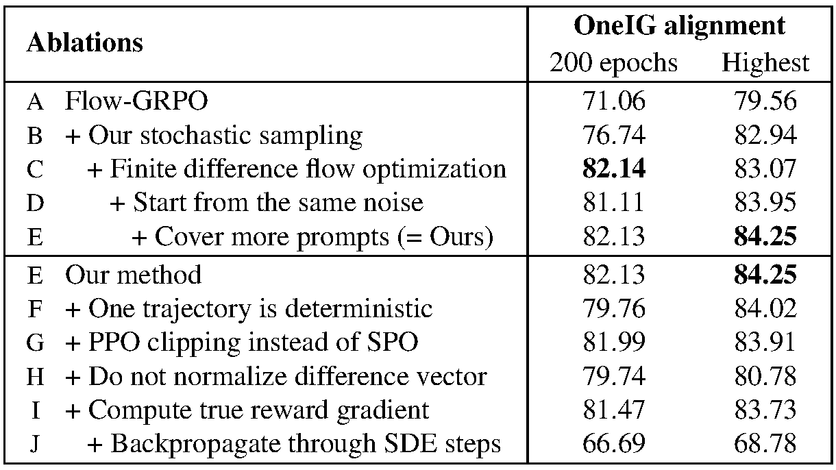
-
Experiments (§5). SD3.5-M on Pick-a-Pic prompts with PickScore, VLM alignment and their sum, against Flow-GRPO at equal cost by reward, OneIG and HPSv2: combined reward 30.3 to Flow-GRPO's 28.5, OneIG alignment 82.13 vs 71.06, one reward in 19× fewer GPU-hours.
-
The exact gradient does not beat the difference (Fig. 8 I–J). The reward model's true gradient for gives 81.47 against 82.13, the smoothing worth the gradient; pushed through the SDE steps it falls to 66.69 — one endpoint direction per step beats per-step credit.
-
Four hours of a human as the reward (§5.6). One author rated 3,200 on-policy pairs in 4 hours, 50 epochs, HPDv2 prompts, no reward model or offline data — possible since one pairwise preference fixes an update direction, a budget the paper calls far too small for Flow-GRPO.
The release pins two things the paper leaves loose and breaks one of its own statements: the pair's shared seed is itself churned, so the pair differs from step one; every loss is a mean over pixels, not the appendix's sum; and the CFG path, KL term and weighting ship, all off in every run.
Advantage Weighted Matching: Aligning RL with Pretraining in Diffusion Models
UCAS · Adobe Research · HKU · MIT
arXiv, 2025
Sep 29, 2025 AWM (51) code (99)
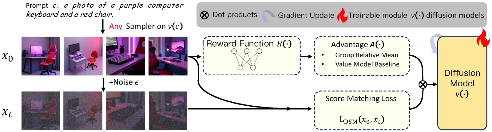
DDPO is denoising score matching with noisy targets; keep the pretraining loss instead and weight each sample by its advantage.
-
The two objectives do not match (§3.2). In LLMs both stages maximize one sequence log-likelihood; in diffusion, pretraining is flow matching on the forward process (Eq. 5) while DDPO, which Flow-GRPO inherits, maximizes a per-step reverse-transition Gaussian likelihood (Eq. 3–4).
-
DDPO is score matching in disguise (Thm 1, Eq. 6). The joint law of is the same forward and reverse, so up to Euler–Maruyama error a DDPO step at targets — denoising score matching conditioned on a noisy intermediate instead.
-
The target is still the right one (Lemma 1). For any , score matching conditioned on has the same population minimizer as the plain objective — the textbook clean-data result is the case — so what separates DDPO from pretraining is not bias but its noise.
-
Noisier conditioning, wider target (Thm 2). Both conditional scores are unbiased, yet conditioning on inflates the target covariance by , where is zero at , climbs strictly with , and diverges as approaches from below.
-
The cost shows without any RL (§3.3, Eq. 7–8). Replace EDM's clean target with the noisy proxy that mirrors DDPO and change nothing else: the run learns in the right direction but reaches every FID level later, so the penalty is the objective, not the RL machinery.
-
A different MDP (§4). DDPO's state is , its action , its policy ; AWM's state is the prompt , its action the finished image , its policy — one decision per finished sample, not one per denoising step, which is what makes the trajectory disposable.
-
The matching loss is the log-likelihood (Eq. 10). is read through its ELBO surrogate ; the uniform beats the ELBO weight of Eq. 2, visual quality and likelihood pulling apart here as they have ever since DDPM.
-
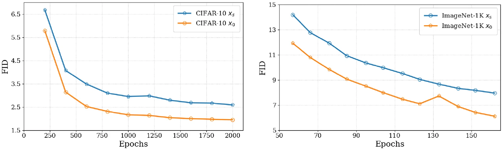
GRPO on that surrogate (Eq. 9, 11–12). The ratio becomes , with and shared across the two policies to cut variance, and the KL a velocity-space — collapses into instability, 2.0 crawls, and 0.4 to 1.0 holds both ends.
-
What the gradient does, and what it frees. On-policy the update is : a positive advantage pulls toward that target, a negative one away. Sampling and training decouple — 20 sampler steps against 4 training ones on its grid, any solver, no CFG.
-
Experiments (§5). SD3.5-M and FLUX with LoRA on GenEval, OCR and PickScore, reward per GPU-hour vs Flow-GRPO: GenEval 0.95 matches it at 8.02× less compute, OCR 0.89 costs 17.6 GPU-hours against 415.9 (23.6×), PickScore 23.02 10.5× less; on FLUX 8.5× and 6.8×.
-
Where is drawn from matters (§5.2, Fig. 7). Uniform and the sampler's grid tie; logit-normal, pretraining's default, lags, then degrades as RL runs on — mid-range mass is the wrong prior once the loss is advantage-weighted; reusing half the last policy's batches changes nothing.
The released configs disagree with the paper on the very knobs the paper reports: the loss is not a plain square, the sampler is not Euler–Maruyama, the training timesteps are six rather than four, and the trust region doing the work is a KL to an EMA copy the paper never names.
# scripts/train_sd3_awm.py with config/dgx_awm.py:geneval_sd3_no_cfg_1node.
# LoRA "default" is v_theta, LoRA "ema" is a slow copy of it, adapters off is v_ref.
x0 = sample["next_latents"][:, -1]  # the rollout, drawn by SA-Solver - not the paper's Euler-Maruyama
t = sample["timesteps"][0][idx] / 1000  # 6 of the sampler's 14 steps, the first dropped; paper says 4 of 20
xt = (1 - t) * x0 + t * noise

# The loss standing in for log pi(x0|c) is neither uniform nor squared: a generalized
# Huber at power 0.25, times t. The paper writes w(t) = 1 and a plain L2.
def log_p(v):  # v = v_theta(xt, t, c), and mse is meaned over every non-batch axis
    return -(((v - (noise - x0)) ** 2).mean(dims) ** 0.25) * t / 0.25

ratio = exp(log_p(v_theta) - log_p(v_old).detach())  # Eq. 11, one t and one noise for both
adv = clip(adv, -5, 5) / 5  # rescaled to +-1, and the std is global, not per prompt
policy_loss = maximum(-adv * ratio, -adv * clip(ratio, 0, 2)).mean()  # clip_range = 1, so barely a clip

# Two KL terms, and the one the paper names carries a thousandth of the weight.
loss = policy_loss + 0.001 * mse(v_theta, v_ref) + 1.0 * mse(v_theta, v_ema)
ema.data = decay * ema.data + (1 - decay) * theta.data  # decay = min(0.3, 0.001 * step)
DiffusionNFT: Online Diffusion Reinforcement with Forward Process
Tsinghua University · NVIDIA · Stanford University
International Conference on Learning Representations (ICLR), 2026
Sep 19, 2025 DiffusionNFT (176) code (1.1K)
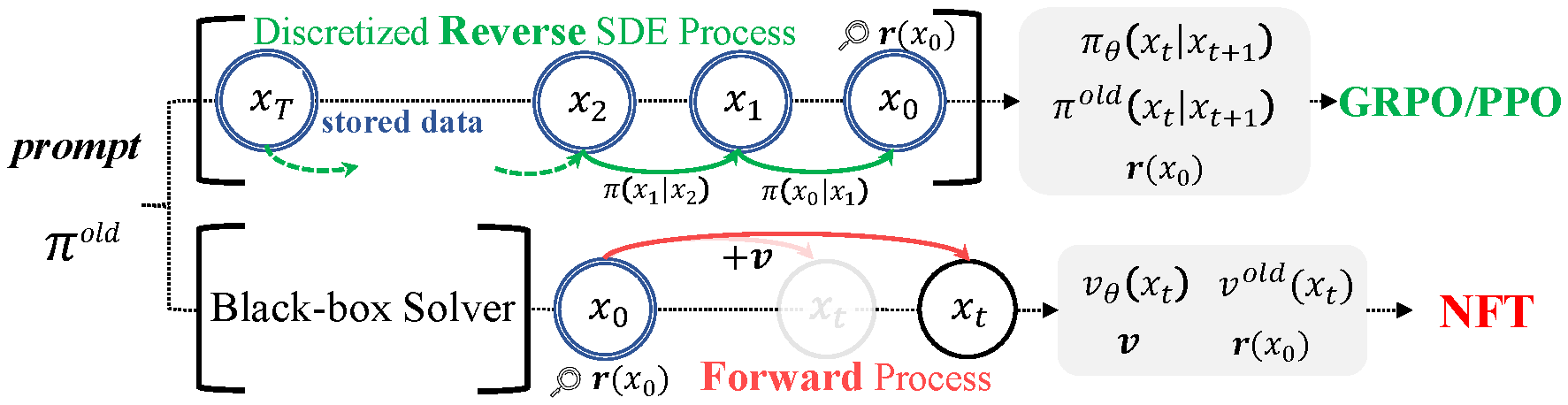
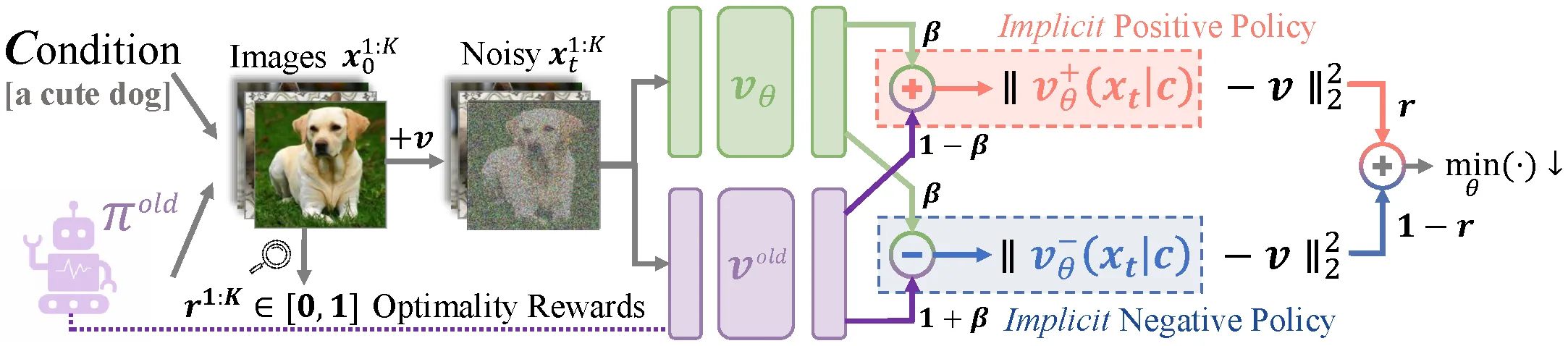
Online RL on the forward process: reward splits the rollouts into implicit positive and negative policies, and one flow-matching loss contrasts them.
-
Why the reverse process is a trap (§2.2). Diffusion admits no exact likelihood, so GRPO-style work discretizes the reverse SDE into tractable Gaussians — a policy gradient bought with first-order SDE samplers, stored trajectories and a model untied from its own forward process.
-
Split the rollouts by reward (§3.1). Read as the probability that a sample is good, . The images then weight two implicit policies, and : each image counts toward the first and toward the second, and .
-
A direction, not a target (§3.2, Eq. 3). Improved velocity : the old velocity plus a correction scaled by — CFG's shape, which the paper reads as the same move, done once and frozen: the conditional model as positive policy, unconditional as negative, as .
-
Why the velocities align (Thm 3.1, Eq. 4). Bayes' rule gives the positive-group probability . The posterior mixture makes : the old velocity lies between the two at fixed noise level, position, and prompt. Thus points toward the positive policy; substituting into gives , the reward-weighted positive policy.
-
One loss, two implicit policies (Eq. 5–6). over has optimum (Thm 3.2): flow matching that has merely seen a reward, the guidance already in it. Delete the negative term and the reward collapses at once (§4.4).
-
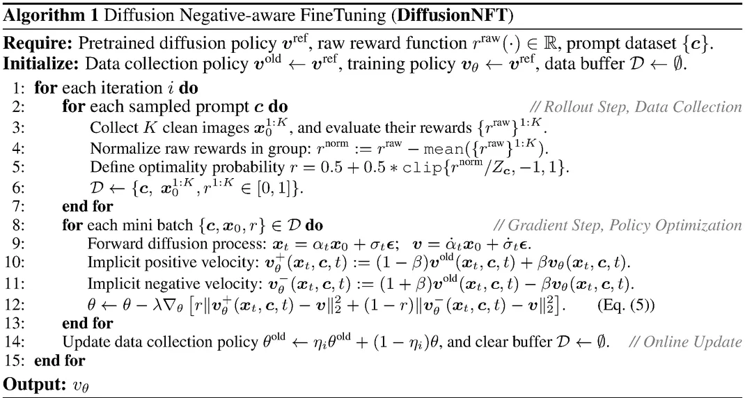
Reward to probability (Alg. 1). with a reward std — group-relative like GRPO, but landing on a split probability rather than an advantage, which is what lets a single batch weight the two branches by and at every noise level.
-
Off-policy by construction (§3.3). The sampler is an EMA copy, , so no importance ratio is needed; on-policy collapses and crawls, while the ramp holds both ends — only the OCR reward needs a 0.999 ceiling.
-
Weighting and guidance strength (§3.3, §4.4). The distillation method DMD's self-normalized regression stands in for the weighting : , beating every fixed schedule while collapses; near 1 is stable, 0.1 buys a faster climb.
-
Solver freedom, and no CFG (§3.2, §4.4). Data collection is a black-box call, so the 2nd-order ODE sampler it permits beats the first-order SDE GRPO is pinned to, clearest on noise-sensitive PickScore; CFG is dropped outright and the policy starts from the conditional model alone.
-
Experiments (§4). CFG-free SD3.5-M (2.5B), five rewards in sequence, preferences first: at 1.7k iterations GenEval 0.94, OCR 0.91, PickScore 23.80, past guided SD3.5-L (8B) everywhere, FLUX.1-Dev (12B) on all but ClipScore; single rewards run 3–25× faster than FlowGRPO.
-
Positives alone collapse (§4.4). Without the reward collapses at once — unlike language models, where rejection-sampling fine-tuning on positives is a strong baseline — so the negative half is what diffusion RL cannot do without — the finding against the LLM playbook.
The released code fills in what the paper leaves out: the three policies are three rank-32 LoRA states of one frozen backbone, the training timesteps are the sampler's own 10-step grid rather than a prior, and an unmentioned anchor on the pretrained model rides along with the objective.
# scripts/train_nft_sd3.py. LoRA "default" is v_theta, LoRA "old" is v_old,
# adapters disabled is the frozen v_ref - one 2.5B backbone, three rank-32 LoRA states.
x0 = batch["latents_clean"]  # rollouts store the clean image only, never the trajectory
t = batch["timesteps"][:, j] / 1000  # t walks the sampler's own 10-step grid, not a prior
xt = (1 - t) * x0 + t * randn_like(x0)  # Alg. 1 line 9, rectified-flow schedule

# Optimality reward, Alg. 1 lines 4-5. Z_c is 5x the per-prompt std, and that std is
# accumulated over the whole epoch's rollouts rather than over the group of 24 alone.
r = clip((adv / 5) / 2 + 0.5, 0, 1)  # adv = clip((r_raw - mean_c) / (std_c + 1e-4), -5, 5)

v_pos = beta * v_theta + (1 - beta) * v_old  # Eq. 5; beta = 1.0, or 0.1 for OCR and multi-reward
v_neg = (1 + beta) * v_old - beta * v_theta

# Adaptive weighting is applied per branch, each normalized by its own error - the paper
# writes one w(t). The velocity is scored through its x0 predictor, never directly.
def nmse(v_hat, dims=(1, 2, 3)):  # per sample, scaled by that sample's own mean error
    e = xt - t * v_hat - x0
    return (e ** 2 / sg(e.abs().mean(dims, keepdim=True).clip(min=1e-5))).mean(dims)

loss = (r * nmse(v_pos) + (1 - r) * nmse(v_neg)).mean() * 5 / beta  # 5/beta pins the step size
loss += 1e-4 * ((v_theta - v_ref) ** 2).mean()  # never in the paper: an anchor on the pretrained model

# Soft update of the sampling LoRA, once per iteration; eta_i = min(0.001 i, 0.5),
# and for OCR min(0.0075 (i - 75), 0.999) - flat for 75 iterations before it ramps.
old.data = eta * old.data + (1 - eta) * new.data
DanceGRPO: Unleashing GRPO on Visual Generation
ByteDance Seed · HKU
arXiv, 2025
May 12, 2025 DanceGRPO (358) code (1.7K)
Concurrent with Flow-GRPO, it took GRPO to production scale across image and video; its shared-noise groups and timestep dropout are stock parts of video RL.
One GRPO recipe stretched across diffusion and rectified flow and across image, video and image-to-video, with the fixes each scale demanded.
-
Diffusion and rectified flow are one update (§2.1). Both read as ; only the meaning of and changes — and for -prediction, and for flow. One MDP then covers both, which is why a single recipe here can span all four base models.
-
Two SDEs, one purpose (Eq. 7–8). Diffusion gets , rectified flow ; under a Gaussian the score is closed-form, so both give a Gaussian policy whose per-step likelihood is as cheap to read as DDPO's.
-
The objective, minus the KL (Eq. 9–10). applied at every timestep because the reward exists only at the last one, inside a clipped ratio. The KL is dropped outright — the paper reports no measurable difference from keeping it, so nothing anchors the policy.
-
One noise per group. All samples for a prompt start from the same . Giving each its own noise, as DDPO does, reliably produces reward hacking and unstable training in video — the group comparison has to be about the policy, not about which seed happened to be lucky.
-
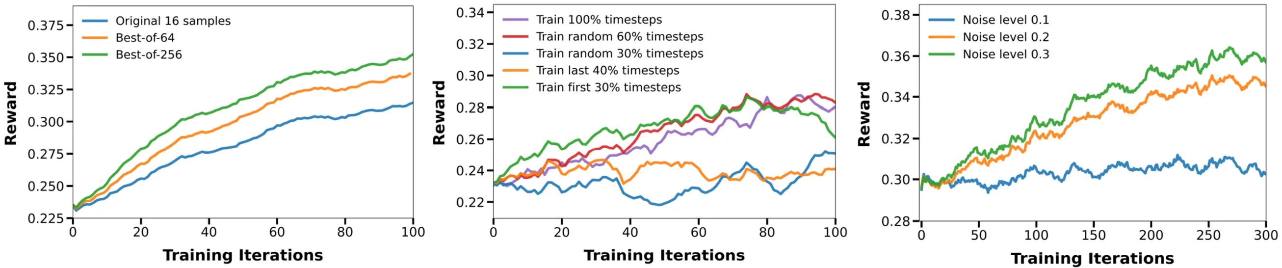
Timestep dropout. 40% of the denoising steps are masked at random each iteration. The first 30% carry the most signal, yet training only on them is worse than the full sequence, so a uniform random subset is the compromise that keeps late-stage refinement in the picture.
-
Several rewards, added as advantages. Reward models live on different scales, so it is the normalized advantages that are summed, , not the rewards. HPS alone drives images toward an oily look; adding CLIP holds them back toward realism.
-
Best-of-N as a data filter (§3.2). Train on the best 8 and worst 8 of a pool of 16, 64 or 256 per prompt: the larger the pool the faster the reward climbs, paid for in sampling time — which is why the paper leaves it an optional extension rather than a part of the default recipe.
-
Binary rewards train (§3.2). Thresholding HPS at 0.28 and CLIP at 0.39 into still moves the model, which is what makes rule-based rewards plausible for images at all, and echoes what verifiable rewards have already done for reasoning in the language models.
-
Experiments (§3). SD1.4, FLUX, HunyuanVideo and SkyReels-I2V on HPS-v2.1, CLIP and VideoAlign, 10K+ prompts: SD1.4 goes 0.239 → 0.365 on HPS, past DDPO's 0.297 and ReFL's 0.357; HunyuanVideo gains 56% visual and 181% motion quality, SkyReels-I2V 91% motion.
-
What it costs, said plainly (§3.2–3.3). Optimizing one reward moves the others: FLUX tuned on HPS alone falls 0.659 → 0.561 on GenEval, and HunyuanVideo's text alignment drops 1.75 → 1.59 while its quality rises — VideoAlign's alignment head was too unstable to train against.
The release fixes the two numbers the paper leaves as symbols, and the noise schedule is not the one its closest neighbour uses.
# fastvideo/train_grpo_flux.py, with scripts/finetune/finetune_flux_grpo_8gpus.sh.
# eta = 0.3 for FLUX, 0.25 for HunyuanVideo, and the step noise is flat in t -
# Flow-GRPO scales its own as a * sqrt(t / (1 - t)).
std_dev_t = eta * sqrt(delta_t)
prev_mean = prev_sample_mean_from(pred, z, sigmas, index, log_term=-0.5 * eta**2 * score)
log_prob = -((z_next - prev_mean)**2) / (2 * std_dev_t**2) - log(std_dev_t) - log(sqrt(2*pi))

# Group advantage, or a global one when --use_group is off.
adv[g] = (rewards[g] - rewards[g].mean()) / (rewards[g].std() + 1e-8)

# The 40% dropout of Section 3.6 is a shuffled index list, truncated.
perms = stack([randperm(len(timesteps)) for _ in range(batch)])
train_timesteps = int(len(timesteps) * 0.6)  # timestep_fraction, one value for every model

ratio = exp(new_log_probs - sample["log_probs"][:, k])
loss = maximum(-adv * ratio, -adv * clip(ratio, 1 - 1e-4, 1 + 1e-4)).mean()  # DDPO's clip range
Flow-GRPO: Training Flow Matching Models via Online RL
CUHK · Tsinghua University · Kuaishou Technology · Nanjing University · Shanghai AI Laboratory
Advances in Neural Information Processing Systems (NeurIPS), 2025
May 08, 2025 Flow-GRPO (570) code (2.5K)
It brought online RL to flow models by turning their ODE into an SDE — the conversion that gave a flow a policy at all, and the start of every flow RL method since.
A flow model has no randomness to explore with — convert its ODE into an equivalent SDE, and GRPO then carries over almost unchanged.
-
The MDP is inherited (§3). , , , reward only at — DDPO's mapping taken whole. What is new is making a flow model fit into it at all, since a flow has no per-step conditional distribution to write down at all, let alone to differentiate.
-
A flow model has no policy (§4). Rectified-flow sampling is the ODE : the step is a bijection, so would need a divergence estimate, and beyond the initial seed there is nothing to explore — given the seed, the trajectory is fixed, every rollout the same.
-
ODE to SDE, the target (App. A, Eq. 10–14). The sampler is the ODE ; wanted is an SDE with the same marginals . Each moves its density by its own law, Fokker–Planck or the continuity equation, so equal marginals means equal right-hand sides:
- The diffusion term is a drift in disguise (Eq. 15–17). Since , : what noise does to is a flow of along its own score. Fold it into the drift and the equation is solved by , an SDE that spreads and re-gathers equally:
- Run it backwards (Eq. 18–21). Generation runs , noise to data, so the reverse-time SDE is what is sampled: Anderson's rule turns into , and with the score's coefficient flips, — the main text's Eq. 7:
- First the score (Eq. 22–24). No network outputs , but for the conditional has score , and the marginal score is its posterior average — , divided through by :
- Then the velocity (Eq. 25–27). ; write and every term is or , which Eq. 24 turns into the score. With , the bracket collapses to , and solving for the score then gives Eq. 27:
- The sampler (Eq. 28–29 = Eq. 8–9). Eq. 27 into the reverse SDE removes the score, and Euler–Maruyama makes every transition a Gaussian: mean the drift step, variance . Time runs , so and the noise scale is , the release's
sqrt(-dt)term:
-
What the Gaussian buys. , the bracket above: the ratio is a quotient of two Gaussian densities and the KL a difference of means, both closed-form, so DDPO's machinery carries over — and the marginals stay the pretrained model's.
-
A KL that costs nothing (§4). Both policies are Gaussians of one variance, so the KL is a squared difference of predicted means — and, as the means differ only through the velocities, of predicted velocities: no second sampling pass, no estimator, no extra gradient variance:
-
The noise level is the exploration knob (§5.3). , which keeps finite at and the noise nil at the data end (my reading): explores too thinly, 0.7 is best, past 1.0 nothing more, and too much noise destroys the samples and the reward with them.
-
The objective (Eq. 4–5). the advantage over a group of images for one prompt, the same scalar at every denoising step, against a per-step clipped ratio and the KL above. No value network appears anywhere, which is the reason GRPO and not PPO.
-
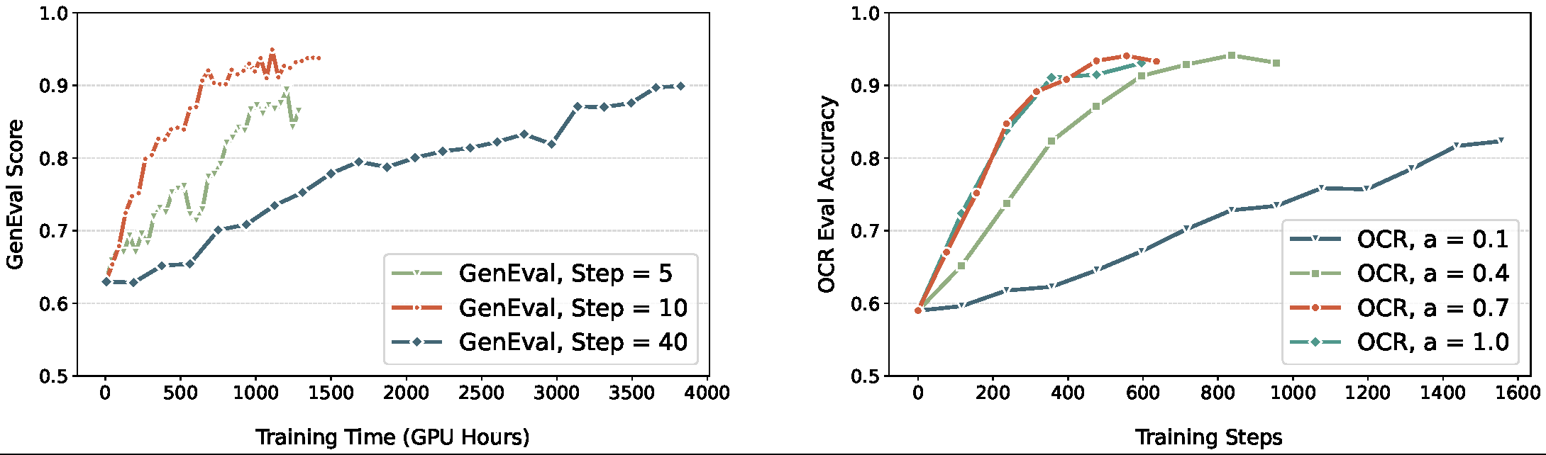
Denoising Reduction. Roll out at and still evaluate at : over 4× faster on all three tasks with no loss in final reward, since low-quality trajectories carry the same ranking signal. Dropping to 5 is not reliably faster and sometimes slower, so ten is where it stops.
-
Group size decides stability (§5.3). trains through; at 12 and 6 the advantage estimate is noisy enough that both runs climb, peak and then collapse outright — a small group makes the denominator of Eq. 4 unreliable long before the numerator itself ever becomes so.
-
Experiments (§5). SD3.5-M on GenEval composition, OCR text rendering and PickScore, DrawBench quality watching for hacking: GenEval 0.63 → 0.95, past GPT-4o's 0.84, OCR 0.59 → 0.92, PickScore 21.72 → 23.31, ahead of SFT, Flow-DPO and their online variants.
-
KL is not early stopping (§5.2–5.3). Without it GenEval still reaches 0.95, but DrawBench aesthetics fall 5.39 → 4.93 and DeQA 4.07 → 2.77; on PickScore, quality holds and diversity collapses instead, different seeds landing on one style — which no early stop would have caught.
-
What a template teaches (§5.3, Tab. 3–4). Trained on 60 GenEval classes and counts of 2–4, it scores 0.90 on 20 unseen classes from 0.64, counts 5–6 objects at 0.48 (0.13), 12 at 0.12 (0.02), and lifts T2I-CompBench 2D-spatial 0.2850 → 0.5447 — relations, not prompts.
The release differs from the paper in the parts a reader would reuse: a second SDE discretization that is not Euler–Maruyama, a filter that throws away prompt groups whose rewards all agree, and an EMA of the trained weights that no section of the paper ever thinks to mention at all.
# scripts/train_sd3.py + flow_grpo/diffusers_patch/sd3_sde_with_logprob.py.
std_dev_t = sqrt(sigma / (1 - sigma)) * 0.7  # the paper's a, pinned to 0.7 as the default
prev_mean = x * (1 + std_dev_t**2 / (2*sigma) * dt) \
          + v_theta * (1 + std_dev_t**2 * (1 - sigma) / (2*sigma)) * dt  # Eq. 9
log_prob = -((x_next - prev_mean)**2) / (2 * (std_dev_t * sqrt(-dt))**2) - log(std_dev_t * sqrt(-dt))

# A second branch nobody writes about: a DDIM-style step whose noise is
# std_dev_t = sigma_prev * sin(a * pi / 2), not the paper's Euler-Maruyama.

ratio = exp(log_prob - sample["log_probs"][:, j])
adv = clip(sample["advantages"][:, j], -5, 5)  # per-prompt std, or a global one by config
policy_loss = maximum(-adv * ratio, -adv * clip(ratio, 1 - 1e-3, 1 + 1e-3)).mean()
kl = ((prev_mean - prev_mean_ref)**2).mean(dims) / (2 * std_dev_t**2)  # the closed form above
loss = policy_loss + 0.04 * kl  # beta = 0.04 for GenEval and OCR, 0.004 in the base config

# Groups where every image scored alike give a zero advantage and are dropped
# before the gradient step; the fraction is logged as zero_std_ratio.
keep = samples["advantages"].abs().sum(dim=1) != 0
Diffusion Model Alignment Using Direct Preference Optimization
Salesforce AI · Stanford University
Conference on Computer Vision and Pattern Recognition (CVPR), 2024
Nov 21, 2023 Diffusion-DPO (863) code (713)
It made preference alignment for image models a fine-tuning job on a static dataset, and became the default first thing to try.
DPO for diffusion — a pairwise preference loss asking only that the model improve on the winner more than it does on the loser beside it.
-
Why not a reward model (§1). RL routes so far tune on small prompt sets and, run against a learned scorer, drift into mode collapse and reward hacking; DPO drops both reward network and rollouts, learning from pairs a reference model drew and people ranked.
-
Bradley–Terry (Eq. 3–4). Preference is a sigmoid of a reward gap, , and a reward net is fit by — plain binary classification on a static, human-labeled dataset, which is all a reward model ever learns.
-
RLHF, and its closed form (Eq. 5–7). Maximize ; the unique optimum is with , so — the reward is a function of the policy and nothing else.
-
DPO (Eq. 8). Put that reward into Eq. 4: cancels across the pair, no reward model is ever fit and no sample is ever drawn, and the policy is trained directly by — the policy is its own reward model.
-
What diffusion breaks (§4, Eq. 9–10). Eq. 8 needs , which marginalizes each path ending at — the one thing a diffusion model never gives. So define a chain reward , , and bound the KL by the joint .
-
The lift, line by line (S2, Eq. 17). Eq. 5 over , sign flipped; each line below is one move — the ELBO bound, the reward swap of Eq. 9, completing the KL with — and the last minimizer is read off: , so , Eq. 7 on paths.
- Path DPO (Eq. 11). into Eq. 4, and cancels again: the first line below is Eq. 8 with path ratios inside an expectation over the reverse process , which is both intractable to sample and steps long. The chain below ( dropped) removes both in turn.
-
Off-policy by substitution (S2, Eq. 18). Line two swaps the unsampleable reverse process for the forward — what lets training run off a fixed dataset — and splits the path ratio into per-step ratios; line three trades the sum over steps for times one random step .
-
Jensen, then KLs (Eq. 12–13). is convex, so the expectation over moves outside it (line four, an upper bound); against the posterior , each ratio's expectation is a difference of two KLs (line five), and every one of them is a Gaussian, by Eq. 1's form.
-
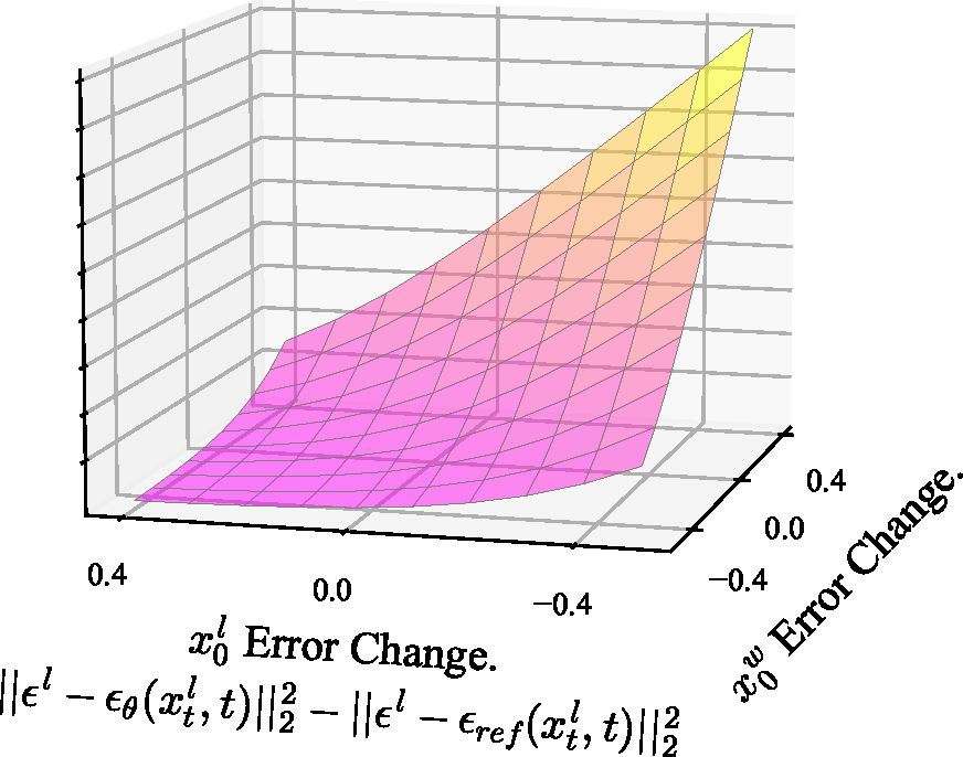
The objective (Eq. 14). Gaussian KLs are squared errors: — four denoising losses at one : denoise the winner better than the reference, the loser worse; folds into , hence a in the thousands.
- The other approximation (S2, ). Per step, stands in for ; using is closer, since — one factor fewer to guess.
-
Why is not the one used. It asks the model to stay near the reference on winners and leave it on losers — but starts at , so both squared differences are zero at initialization and so is the gradient, whereas has the data's to pull against from the very first step.
-
A noisy classifier gives it too (S4, Eq. 44–46). Condition the policy on ; with the DDIM likelihood , each log-ratio in Eq. 8 is a gap in squared noise error times , so — Eq. 14, and the code's .
-
The same MDP as DDPO, solved off-policy (S3, Eq. 19–23). State , action , reward at ; soft optimal control gives , exact since the right side integrates to one, so exactly, Eq. 25.
-
Telescoping to Eq. 11 (Eq. 24–27). The inverse Bellman equation (Eq. 24), summed down the chain, leaves ; cancels across a pair — Eq. 11, reached with no rollout at all.
-
Data and the scaling rule (§5.1). Pick-a-Pic v2: 851,293 pairs over 58,960 prompts once the ~12% ties are dropped; batches of 2048 pairs; for SD1.5 and for SDXL, learning rate , 25% warmup — scaling, since the gradient's norm grows with .
-
Experiments (§5). SD1.5 and SDXL-base tuned on Pick-a-Pic v2, five labelers on PartiPrompts and HPSv2: DPO-SDXL beats SDXL-base 70.0% / 64.7%, appeal and alignment moving in step, and the 6.6B base+refiner 69% / 64% from 3.5B; and wins TEdBench edits 65% to 24%.
-
A reward model falls out for free (§5.5, Tab. 2). The inner term of Eq. 14, averaged over 10 random , estimates a reward gap, so the tuned model is also a preference classifier: DPO-SDXL scores 72.0% on Pick-a-Pic v2 validation, above PickScore's 64.2, HPS's 59.3 and CLIP's 57.1.
-
Pseudo-labels beat labels; SFT hurts SDXL (§5.4–5.5). Reranking pairs by PickScore, not people, lifts the PartiPrompts win rate 59.8% → 63.3%; fine-tuning on winners alone helps SD1.5 (55.5%) yet hurts SDXL at any rate: SDXL-1.0 already outdraws the models that made the data.

The released code tracks the paper closely, but three of its own lines carry decisions that the derivation in Section 4 never mentions at all.
# train.py from the official Salesforce release. The pair arrives concatenated
# along the channel axis and is split apart; the winner is the first half.
timesteps = timesteps.chunk(2)[0].repeat(2)  # one t for the pair, not two - never stated in Eq. 14
noise = noise.chunk(2)[0].repeat(2, 1, 1, 1)  # and one epsilon, which halves the gradient noise

model_losses = (model_pred - noise).pow(2).mean(dim=[1, 2, 3])
model_diff = model_losses_w - model_losses_l  # the model's margin
ref_diff = ref_losses_w - ref_losses_l  # the frozen reference's margin, no grad

# omega(lambda_t) is dropped outright; the -beta/2 is Eq. 46's coefficient, b_t^2/(a_t^2 sigma_t^2) ~ 1.
inside_term = -0.5 * beta_dpo * (model_diff - ref_diff)  # beta_dpo = 5000 by default
loss = -F.logsigmoid(inside_term).mean()
implicit_acc = (inside_term > 0).float().mean()  # the implicit reward model, scored live

# AI feedback (5.4) is this one line: a scorer reorders the pair before training.
if choice_model_says_flip(batch): feed_pixel_values = feed_pixel_values.flip(0)
DPOK: Reinforcement Learning for Fine-tuning Text-to-Image Diffusion Models
Google Research · University of Wisconsin-Madison · UC Berkeley · Amazon · KAIST
Advances in Neural Information Processing Systems (NeurIPS), 2023
May 25, 2023 DPOK (483) code
Concurrent with DDPO, it supplied the other half of diffusion RL — a KL to the pretrained model in the objective, the anchor later methods keep, tune, or argue away.
The same multi-step MDP as DDPO, arrived at independently, and a KL to the pretrained model carried the whole way as an implicit reward.
-
The MDP, indexed backwards (Eq. 4). , , , transitions , , reward only at — the same mapping DDPO found, written so that MDP time runs forward while the denoising runs backward.
-
The objective and its gradient (Eq. 5–6). Minimize ; Lemma 4.1 turns that into , REINFORCE over the -step chain. The DDPM covariance stays frozen at and only is trained, which is what leaves the policy stochastic.
-
A KL you can actually compute (Lemma 4.2, Eq. 7). The divergence that matters is on the image, and that marginal is intractable — so bound it over all steps by , which makes every term a Gaussian KL with a closed form of its own.
-
The regularized objective (Eq. 8). — and trade reward against drift, and the KL arrives as a second reward evaluated online, per update, on fresh samples, which is precisely the thing a supervised fine-tuning pass cannot do.
-
The gradient they actually use (Eq. 9) is not that objective's. differentiates the KL's value but not the state distribution that the KL is measured under — a gap the main text flags plainly in the line right after the equation, not in the code.
-
The term they drop (App. A.3, Eq. 16). The KL sits under , the policy's own state distribution, so the product rule adds a second term, : each step then carries the KL of every step still ahead of it, dropped purely for its cost.
-
Reusing a round of samples (App. A.6, Eq. 25–26). Writing for the sampling policy, a ratio against it lets five gradient steps run off one round, and a PPO clip bounds the drift: , with a learned value baseline that cuts variance.
-
KL for supervised fine-tuning too (Eq. 10–13). The baseline is ; Lemma 4.3 bounds its KL-regularized form two ways — KL-D shifts the weight to , smoothing it toward uniform, and KL-O adds , pinning the denoising direction to the pretrained one.
-
Three ways online differs (§4.3). RL may search outside the pretrained support while SFT only imitates inside it; RL's KL is measured on new samples each update, SFT's on a frozen set; and RL queries the reward model off-distribution, so it inherits whatever that model generalizes.
-
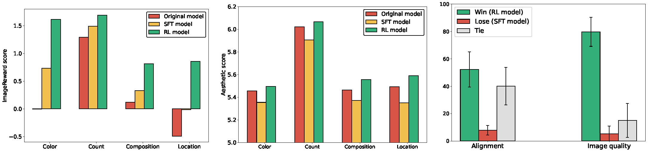
Experiments (§5). SD v1.5, LoRA, ImageReward reward, one prompt per color, count, composition and location, judged by ImageReward, aesthetics, raters: RL beats SFT on all four, aesthetics intact; on 104 COCO / 183 DrawBench prompts it goes 0.22 → 0.55 / 0.13 → 0.58.
-
Whiskey to flowers (§5.4). "Four roses" draws the whiskey from the base model; RL against ImageReward turns it into the flower, the score rising −0.52 → 1.12 — human feedback undoing a bias the web corpus put in, the clearest case for a preference model over a caption.
The release fixes what the paper leaves as symbols, and one of those numbers openly disagrees with the value its own appendix reports.
# dpok/train_online_pg.py from google-research. alpha and beta of Eq. 8 are
# flags: reward_weight defaults to 100, though App. B reports alpha = 10.
log_prob, kl_regularizer = pipe.forward_calculate_logprob(..., unet_copy=unet_copy)

# v_flag off by default: the "advantage" is the raw reward, uncentred - no
# per-prompt baseline of the kind DDPO normalizes with.
adv = reward - value_function(x_t, txt_emb, t) if v_flag else reward

# Not PPO. The ratio is clamped outright, so a sample outside the trust region
# contributes a constant instead of being discarded by a max() over two branches.
ratio = clamp(exp(log_prob - old_log_prob), 1 - 1e-4, 1 + 1e-4)
loss = (-100.0 * adv.detach() * ratio).mean()
if step > kl_warmup: loss += 0.01 * kl_regularizer.mean()

# log_prob is meaned over the latent axes, not summed, so its scale depends on
# resolution - part of why the reward weight has to be so large.
Training Diffusion Models with Reinforcement Learning
UC Berkeley · MIT
International Conference on Learning Representations (ICLR), 2024
May 22, 2023 DDPO (1,035) code (776)
The multi-step MDP it defines is the formulation every later diffusion RL method either builds on or argues against.
Read denoising as a multi-step decision process, and each sampler step becomes a Gaussian whose exact likelihood a policy gradient can use.
-
The objective training never optimizes (§4.1). A diffusion model is fit to a data distribution, but the goal is for a black-box reward — and is the one quantity a diffusion model cannot evaluate, since it marginalizes every denoising path.
-
Reward-weighted regression (§4.2). Collapse sampling to a one-step MDP (, ) and reweight the denoising loss by — no heuristic, since the KL-constrained optimum is and fitting to that optimum is reward-weighted maximum likelihood.
-
Except the likelihood is a bound (§4.2). That derivation needs itself, and a diffusion model's bound falls short of it by exactly — a divergence conditioned on that image, so the slack differs sharply from one sample to the next.
-
What the slack costs (App. E.2). The ratios reach the gradient scaled by an unknown factor, and the loss can fall by shrinking that slack instead of the likelihood — effort the reward pays for and the image never sees. RWR fed 16,384 samples a round never catches up.
-
Denoising as a multi-step MDP (§4.3). Choose what counts as an action and the rest of the mapping follows. Writing for a Dirac mass at , the transitions here are deterministic and starts every rollout at step from pure noise, so all of the trajectories share one horizon.
| RWR, one step (§4.2) | DDPO, multi-step (§4.3) | |
|---|---|---|
| State | ||
| Action | ||
| Policy | ||
| Transition | straight to an absorbing state | |
| Initial state | ||
| Reward | at , else |
-
The return is the reward (§4.3). Only the final step pays and nothing is discounted, so a whole trajectory returns exactly : maximizing in this MDP and maximizing are literally the same problem, which is what licenses a policy gradient estimator here at all.
-
Why that buys exact likelihoods. Under a standard sampler the policy is the isotropic Gaussian : per-step log-likelihoods and their gradients are exact, where the marginal over all of the many trajectories that could reach a given never is.
-
The score function estimator, (§4.3). — REINFORCE, the one terminal reward multiplying every step's score. The expectation runs over the current 's own trajectories, so a round of data buys exactly one gradient step.
-
The importance-sampled estimator, (§4.3). — the expectation now runs over 's trajectories, so several updates fit one round; it decays as drifts, which the clipping bounds.
-
The clip range has to be tiny (App. D.5). 1e-4, four orders below what standard RL tasks use — the per-step Gaussians sit so close together that an ordinary trust region is no constraint at all, and rewards are normalized per prompt by a running mean and standard deviation.
-
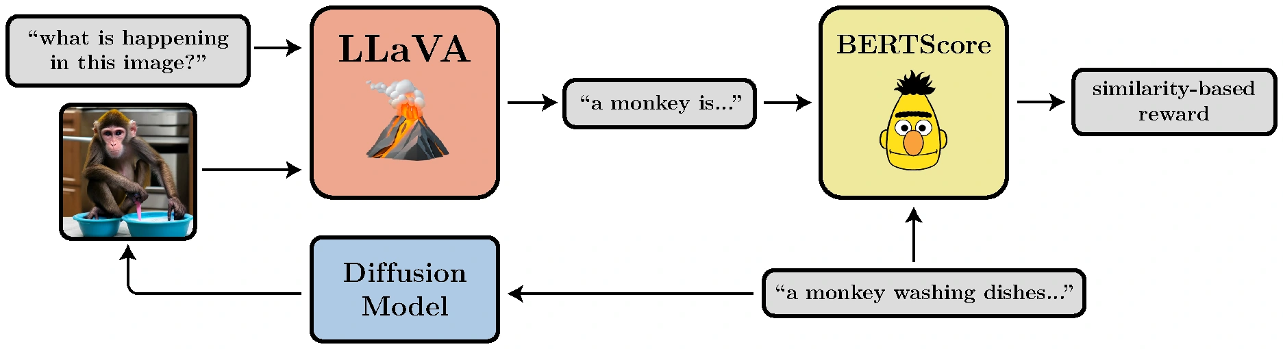
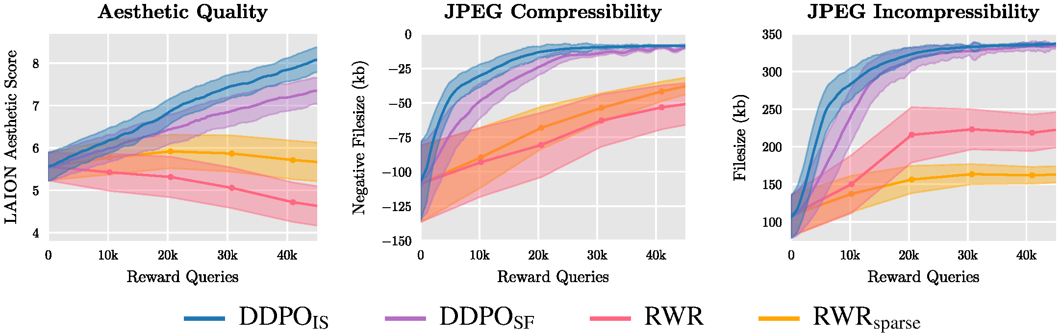
Experiments (§6). SD v1.4 on four rewards — (in)compressibility over 398 animals, LAION aesthetics over 45, LLaVA alignment over 45 × 3 activities — reward per query: both DDPO variants beat both RWRs, IS ahead of SF, and alignment climbs on prompts the base never solved.
-
Every reward has a style tax (§6). Aesthetics turns photos into drawings, compressibility strips backgrounds, incompressibility adds noise, alignment goes cartoon-like unasked — the pretraining prior, or the VLM liking cartoons; and it transfers to unseen animals and objects.
The PyTorch release pins what the paper leaves to a table, and the choice that matters most is the one that makes the policy stochastic at all.
# scripts/train.py + config/base.py from the official ddpo-pytorch release.
# eta = 1.0: DDIM run at full DDPM noise, since eta = 0 is deterministic and a
# deterministic policy has no log-likelihood to take a gradient of.
noise_pred = uncond + 5.0 * (text - uncond)  # trained on the guided prediction, App. E.1
_, log_prob = ddim_step_with_logprob(scheduler, noise_pred, t, x_t, eta=1.0, prev_sample=x_next)

adv = clip(sample["advantages"], -5, 5)  # per-prompt running mean/std over a 16-sample buffer
ratio = exp(log_prob - sample["log_probs"][:, j])  # one ratio per denoising step, not per image
loss = maximum(-adv * ratio, -adv * clip(ratio, 1 - 1e-4, 1 + 1e-4)).mean()
Reward Modeling
Improving Video Generation with Human Feedback
CUHK · Tsinghua University · Kuaishou Technology · SJTU · Shanghai AI Laboratory
arXiv, 2025
Jan 23, 2025 VideoReward (255) code (505)
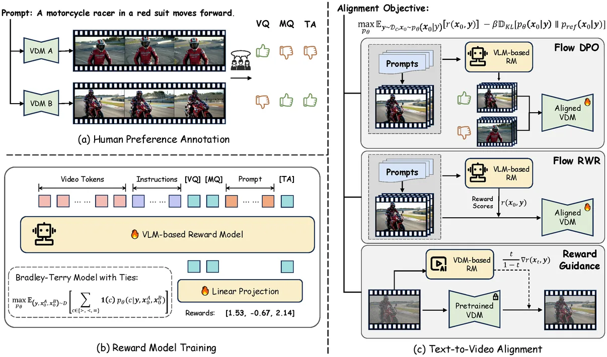
A 182k pairwise video preference set and the reward model it trains, then DPO, RWR and reward guidance carried across to flow models.
-
The gap being filled (§1, §3.1). Existing video preference sets score pre-Sora generators — short clips, visible artifacts. This one annotates 12 modern models into 182k triplets on visual quality, motion quality and text alignment, three annotators each and a fourth when they disagree.
-
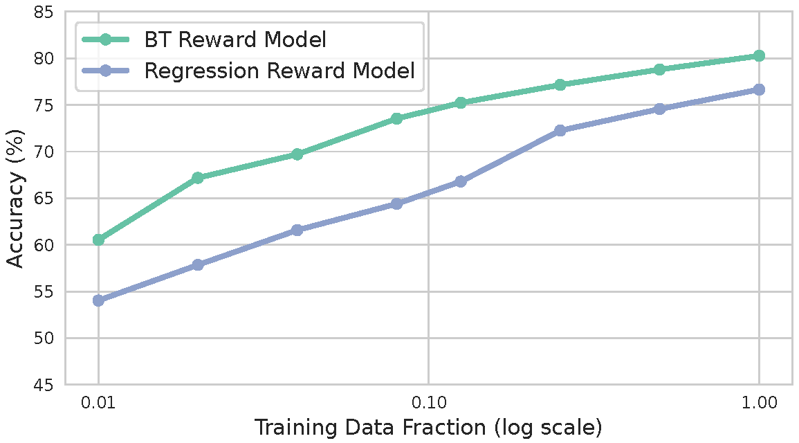
Pairwise beats pointwise (§3.2). The same annotators labeled the same videos both ways, so the comparison is clean: Bradley–Terry on pairs beats regression on 1–5 scores at every data fraction. Raters agree on which is better far more readily than on a number out of five.
-
Ties are data, not noise (§3.2). Plain Bradley–Terry throws tied pairs away; the with-ties extension models them, and the ties-included accuracy rises from 61.22 to 61.50 while ties-excluded goes 72.58 → 73.39 — the tied cases are what teach the model where its boundary lies.
-
The reward model (§3.2, §5.1). Qwen2-VL-2B, LoRA on the language model's linear layers with the vision encoder fully trained; a separate token per axis rather than one pooled last token; 2 fps at about 448×448, batch 32, lr 2e-6, two epochs, roughly 72 A800 hours.
-
Flow-DPO (Eq. 8–10). For rectified flow , so Diffusion-DPO's noise-space loss becomes a velocity-space one otherwise unchanged — except that the KL coefficient picks up a schedule, , falling straight out of that same substitution.
-
And the schedule is the wrong one (§4.1, §5.2). loosens the constraint exactly where the noise is highest, so the model aligns hardest where the signal is worst: VBench drops to 80.90 and text alignment to a 28.14 win rate. Holding constant gives 83.41 and 68.26.
-
Flow-RWR (§4.2). The same KL-regularized optimum , read as an EM step and simplified to with rewards normalized to zero mean and unit variance. It lands between SFT and Flow-DPO on every benchmark and beats neither of them.
-
Flow-NRG (§4.3). Guide at inference instead: tilts the marginal toward , so weights over the three axes become a runtime dial. It needs a reward on noisy video, fitted by Bradley–Terry on noised pairs and read off the generator's own first 20 blocks.
-
Experiments (§5). The reward model on VideoGen-RewardBench (26.5k new pairs), accuracy with/without ties: 61.26 / 73.59 against VisionReward's 56.77 / 67.59; alignment by VBench and reward win rates — Flow-DPO 83.41 and 93.42 / 69.08 / 75.43 on VQ / MQ / TA.
-
LoRA is a requirement, not a shortcut (§5.2). Full-parameter fine-tuning degrades or collapses the model, on all three algorithms. The training set is relabeled by VideoReward before alignment, so scoring the result with VideoReward is at least self-consistent rather than circular.
-
Guidance weights are a runtime dial (§5.2, Tab. 6–7). VQ:MQ:TA at 0:0:1 lifts TA to 70.42, 0.5:0.5:0 lifts VQ / MQ to 86.43 / 93.23, no retraining; a reward head fit on clean latents fails on noisy ones (37.1 / 38.6 against 66.2 / 74.6), and predicting first breaks the video.
Only the reward model is released — the three alignment algorithms are not — and it pins a constant the paper leaves as a symbol, while shipping four extra preference losses that no section of the paper mentions, no table in it reports and no ablation anywhere in the paper ever touches.
# trainer.py from KwaiVGI/VideoAlign. Rewards come from the special-token
# positions, one per dimension, not from the pooled last token.
pooled = logits[input_ids == special_token_ids, ...]  # reward_token = "special"

# Bradley-Terry with ties. theta is the tie band; the paper leaves it a symbol.
k = 5.0                       # <- never stated in the paper
bt   = -logsigmoid(r_chosen - r_rejected - log(k))
same = -logsigmoid(r_chosen - r_rejected - log(k)) \
       -logsigmoid(r_rejected - r_chosen - log(k)) - log(k**2 - 1)
loss = bt * nontied_mask + same * (1 - nontied_mask)

# Four more losses ship unused: a margin BT that subtracts the annotators' own
# score gap, a constant margin of 0.57, a margin-scaled BT, and plain regression
# against (score - 3.0). Only "btt" is the one the paper reports.
Last updated on September 17, 2026 · Citations from Semantic Scholar & Google Scholar; stars from GitHub, September 2026