Efficiency & Systems
Making training and inference fit the compute you actually have.
8 papers
Written by Junkun Yuan.
Click here to go back to main contents.
Table of contents ▶
Papers are displayed in reverse chronological order. High-impact or inspiring works are highlighted in red.
Distillation
Large Scale Diffusion Distillation via Score-Regularized Continuous-Time Consistency
Tsinghua University · NVIDIA
International Conference on Learning Representations (ICLR), 2026
Oct 09, 2025 rCM (66) code (803)
It scales continuous-time consistency distillation to 14B video models and fixes its fine-detail failures with a score distillation regularizer.
-
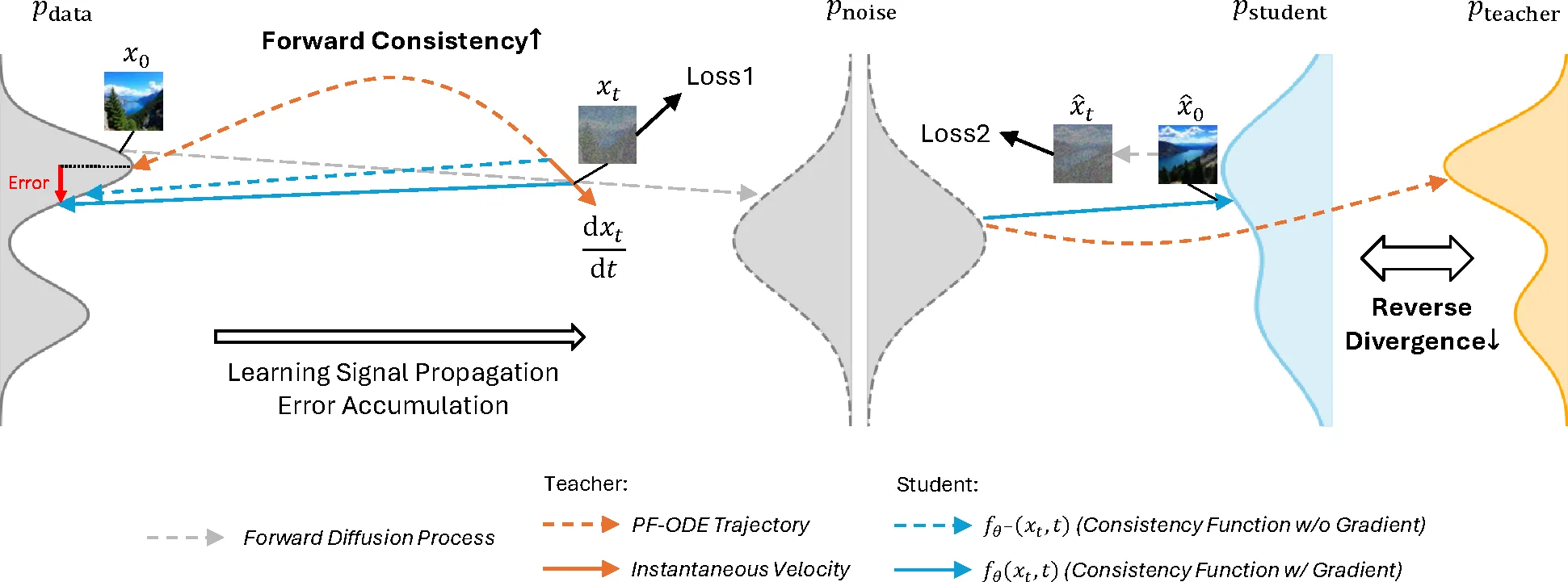
Any teacher, wrapped into TrigFlow (§3.1, Eq. 3). A consistency function maps any point of the teacher's trajectory to its start; on it is , so predicts velocity. For a rectified-flow teacher, solving gives a time map and the wrapped pair , , FP64, no retraining.
-
The sCM loss, stripped down (§3.1, Eq. 4). With , the tangent of the stop-gradient student along the teacher ODE, , , folded into the JVP. sCM's adaptive weighting goes — the normalized loss sits near 1 anyway — and so do its Fourier-embedding and AdaGN fixes: these DiTs keep positional time embedding, AdaLN and QK-norm.
-
JVP at scale (§3.2, App. C, Alg. 2). The tangent is one forward-mode pass through the whole DiT. A Triton FlashAttention-2 kernel streams the output tangent in the same tiled loop as the output, , ; every layer takes and returns tangents, so FSDP shards at layer boundaries; context parallelism all-to-alls tangents like activations — JVP training past 10B parameters, a first.
-
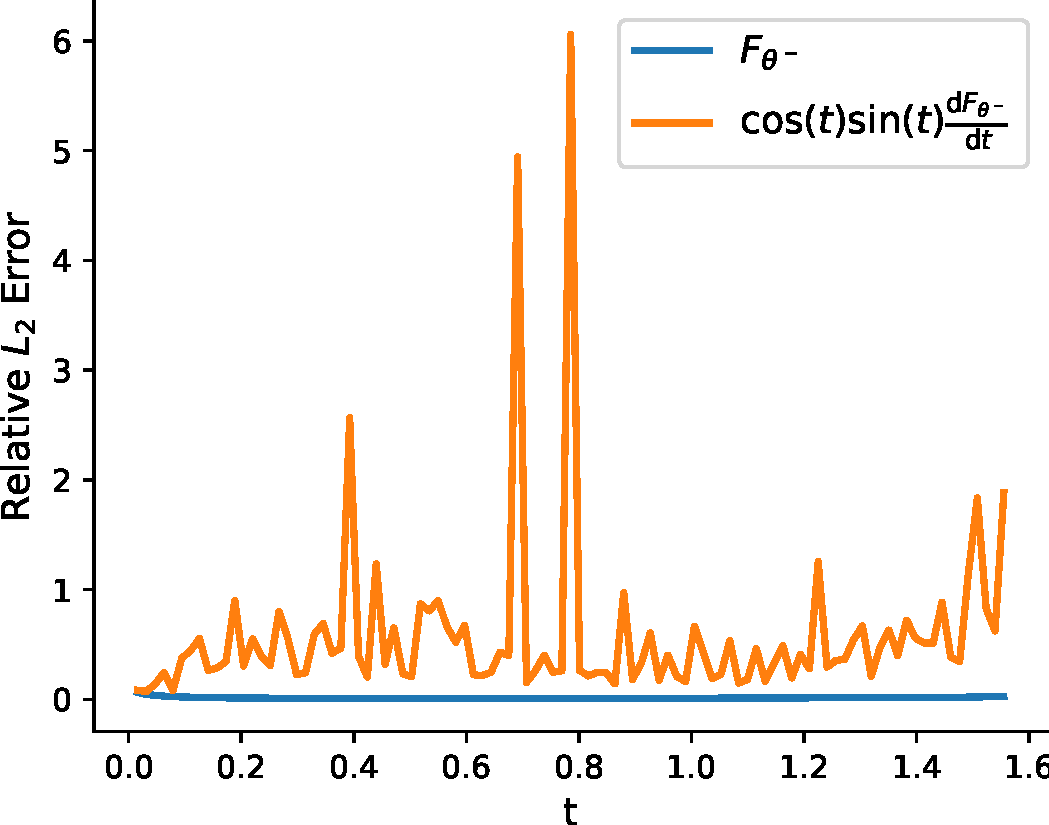
Where pure sCM breaks (§3.3, Eq. 5). The target expands to : the teacher's term fades as and the JVP self-feedback rules the noisy end, where BF16 leaves it a relative error near 6 against ~0 for (Fig. 11). Errors walk from small to large : easy prompts stay sharp, but small text and cross-frame object geometry distort, at 14B too (Fig. 3).
-
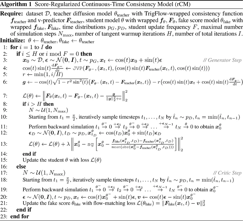
Score regularization (§4.1, Eq. 6). On samples re-noised to , DMD's reverse-KL gradient is a regression carrier, , both read at , a teacher copy refit on those samples (line 21).
-
One objective, two divergences (§4.1). , throughout: the forward, offline signal covers modes and blurs; the reverse, on-policy one seeks modes and sharpens — the long skip above. DMD over SiD's Fisher divergence: no edge here, less memory.
-
Rollout (§4.1, Alg. 1 lines 9–11). Sampling alternates denoise and re-noise, , , gradient through the last step only, times , — decreasing at random, so the full range is covered; DMD2 pins fixed steps.
-
Stable time derivative (§4.2). The JVP collapses late in training through , the oscillating time embedding. Semi-continuous time: exact JVP for the half, a finite difference , , for the rest — enough for 2B images. High-precision time: the full JVP with every time-embedding layer held in FP32 — what 10B+ and video need.
-
The loop (Alg. 1, App. D). Student and fake score start as the teacher with CFG 4.5 / 5 distilled in, full-parameter, no LoRA; one student step per critic steps (10 at 14B); no gradient clipping, called crucial. Sampling walks , trading quality for diversity.
-
Experiments (§5). Cosmos-Predict2 T2I by GenEval and Wan2.1 T2V by VBench, 4 steps against 35×2 / 50×2 teachers and DMD2: GenEval 0.83 at 14B to the teacher's 0.84, VBench 84.92 to 83.58; level with DMD2 at 1.3B (84.43 vs 84.56), 15–50× faster, diversity intact.
-
The quality metric cannot see the collapse (§5.2, Fig. 7). Sweeping on Wan 1.3B moves VBench only 84.32 / 84.57 / 84.43 / 82.68 while diversity visibly falls with every step up; the sweet spot 0.01 is the smallest that still holds quality, picked by eye.
-
MeanFlow's second clock hurts distillation (App. F.1, Fig. 10). sCM with a second time , predicting jumps — MeanFlow in TrigFlow time — trails plain sCM in both quality and diversity on basic T2I: every jump along the trajectory is harder to learn than the one to .
The algorithm and its code. The release distills Wan2.1 only; t2v_model_distill_rcm.py follows Alg. 1 line by line, its departures being the quiet ones — the tangent norm, a cycled step count, the critic loss in units; the 14B config also shifts a full unit noisier than Table 4 and drops the tangent warmup to zero iterations — and its README now advises staging dCM → sCM → DMD+sCM when joint training turns unstable.
# t2v_model_distill_rcm.py, condensed. Student and fake score both load the teacher's weights;
# every F-th iteration is a student step (F = 5 at 1.3B, 10 at 14B), the rest train the fake score.
def scm_step(x0, cond, it):  # Alg. 1 lines 3-7
    # p_G: lognormal sigma, arctan'd into TrigFlow time; mean 0.7 at 1.3B is Tab. 4's -0.8 + log sqrt(T),
    # the 14B config moves it to 1.5.
    t = rf_to_trig_time(p_G.sample())
    x_t = cos(t) * x0 + sin(t) * randn_like(x0)
    with no_grad():
        F_t = denoise("teacher", x_t, t, cond).F  # CFG at scale 5 folded in: F_u + 5 * (F_c - F_u)
        # Line 4, JVP rearrangement: tangents cos t sin t F_teacher and cos t sin t. fd_type=1
        # swaps the time half for the finite difference of §4.2; the Wan configs keep fd_type=0.
        _, dF = denoise_withT("student", (x_t, cos(t) * sin(t) * F_t), (t, cos(t) * sin(t)), cond)
    F_s = denoise("student", x_t, t, cond).F; F_sg = F_s.detach()
    r = min(1, it / H)  # tangent warmup, line 5: H = 1000 at 1.3B, 0 at 14B (Tab. 4 says 200)
    g = -cos(t) * sqrt(1 - r**2 * sin(t)**2) * (F_sg - F_t) - (r * cos(t) * sin(t) * x_t + dF)
    g[isnan(g)] = 0  # a BF16 JVP that overflowed zeroes its sample instead of the run
    g = g / (g.norm() + 0.1)  # Eq. 4 prints ||g||^2 + c; the code divides by ||g||
    return 100 * ((F_s - F_sg - g) ** 2).sum()  # loss_scale 100 : loss_scale_dmd 1, lambda = 0.01

def rollout(cond, n, with_grad):  # lines 10-11: t_1 = pi/2, then t_n = min(t_hat ~ p_D, t_{n-1})
    x, t = randn(shape), pi / 2
    for i in range(n):
        with (enable_grad if with_grad and i == n - 1 else no_grad)():
            x = denoise("student", x, t, cond).x0  # gradient through the final denoise only
        if i < n - 1:
            t = minimum(rf_to_trig_time(p_D.sample()), t); x = cos(t) * x + sin(t) * randn_like(x)
    return x

def dmd_step(cond, it):  # lines 9-13, Eq. 6
    x0_s = rollout(cond, n=it % 4 + 1, with_grad=True)  # N cycles 1, 2, 3, 4; Alg. 1 draws it
    t = rf_to_trig_time(p_D.sample()); x_t = cos(t) * x0_s + sin(t) * randn_like(x0_s)
    with no_grad():
        x0_fake = denoise("fake", x_t, t, cond).x0; x0_teach = denoise("teacher", x_t, t, cond).x0
        weight = (x0_s - x0_teach).abs().mean().clip(min=1e-5)
    grad = (x0_fake - x0_teach) / weight
    return ((x0_s - (x0_s - grad).detach()) ** 2).sum()  # a carrier: its gradient is grad

def critic_step(cond, it):  # lines 17-21
    x0_s = rollout(cond, n=it % 4 + 1, with_grad=False)
    t = rf_to_trig_time(p_D.sample()); x_t = cos(t) * x0_s + sin(t) * randn_like(x0_s)
    x0_fake = denoise("fake", x_t, t, cond).x0
    return ((x0_s - x0_fake) ** 2 / sin(t) ** 2).sum()  # ||F_fake - v||^2, written in x0 units
Improved Distribution Matching Distillation for Fast Image Synthesis
MIT · Adobe Research
Advances in Neural Information Processing Systems (NeurIPS), 2024
May 23, 2024 DMD2 (652) code (1.5K)
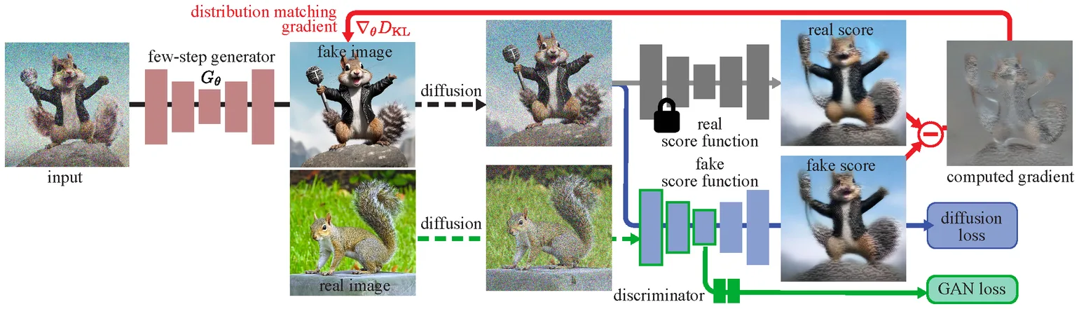
It frees DMD from its regression loss, adds a GAN head trained on real images, and lets a few-step student beat its own teacher.
-
What the regression loss cost (§3). DMD stabilized training by regressing the student onto precomputed teacher ODE pairs: about 700 A100-days of pairs for SDXL — over 4x DMD2's whole training budget — and a leash to the teacher's sampling paths that caps it at teacher quality.
-
Two time-scale update rule (§4.2). Drop it naively and stability goes too — brightness oscillates — because tracks the generator's shifting output too loosely. Five fake-score updates per generator update restore DMD's ImageNet FID, 3.48 to 2.61, with no paired data.
-
A GAN head on the fake score (§4.3). What remains is the teacher's approximation error, unfixable while the student never sees real data. A classifier on 's mid-block judges noised real vs. fake (Eq. 4): 2.61 to 1.51, then 1.28 trained longer — past the teacher itself.
-
Multi-step generator (§4.4). Four timesteps, 999/749/499/249, identical at training and inference; sampling alternates denoising with re-noising. SDXL is the motivation: one step cannot carry the noise-to-megapixel map — its one-step model kept a 10K-pair warmup (App. J.4).
-
Backward simulation (§4.5). Earlier multi-step students train on noised real images, yet from step two onward inference feeds them their own outputs. DMD2 makes training inputs by running the student itself — cheap at few steps — and SDXL patch FID falls 24.21 to 20.86.
-
One loop, three players (Alg. 7). Every iteration updates the fake score and discriminator; every fifth, the generator, on matching gradient plus weighted GAN loss. Neither half suffices alone: pure GAN gets 2.56. One-step SD v1.5: COCO FID 8.35, past its 50-step teacher.

-
Experiments (§5). ImageNet-64 by FID, COCO by FID, patch FID and CLIP, distilling EDM, SD v1.5 and SDXL on 3M LAION prompts: one step 1.51 on ImageNet, past the teacher's ODE 2.22; four-step SDXL 19.32 FID / 0.332 CLIP against the teacher's 19.36 / 0.332 at 100 steps.
-
Pure GAN wins FID and loses the picture (Tab. 4). Without distribution matching, SDXL FID is the lowest, 13.77, and CLIP the worst, 0.307: the real distribution is matched while alignment and aesthetics go, and CFG cannot be taken — why patch FID and raters carry the claim.
Fast High-Resolution Image Synthesis with Latent Adversarial Diffusion Distillation
Stability AI
SIGGRAPH Asia, 2024
Mar 18, 2024 LADD (310)
Distillation goes fully latent — the teacher generates the training data, its features judge real from fake, and the distillation loss goes obsolete.
-
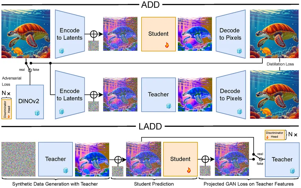
What ADD paid for pixels (§3). ADD decodes latents back to images for both of its losses — a DINOv2 discriminator and a pixel-space distillation term — which costs memory and caps resolution. LADD never leaves the latent space, and megapixel multi-aspect synthesis follows.
-
The teacher becomes the discriminator (§3). Generated latents are re-noised at a logit-normal and fed through the frozen teacher; discriminator heads sit on the token sequence after every attention block of the teacher itself, conditioned on noise level and pooled CLIP text.
-
Synthetic data retires the distillation loss (§4.2). Training images come from the teacher at one fixed CFG scale, so image-text alignment is uniformly high; on them an added distillation term — which still helps real data — buys nothing, and the adversarial loss alone suffices.
-
Scaling, then the product (§4–5). In the three-way scaling study the student's size matters most; LADD distills the 8B MMDiT into SD3-Turbo — megapixel multi-aspect images in four unguided steps that match state-of-the-art text-to-image models, with DPO layered on top.
-
Experiments (§4–5). Ablations on a 2B MMDiT by CLIP on DrawBench and PartiPrompts; 8B SD3-Turbo by raters: one step beats every baseline on both axes, four steps ties 50-step SD3 on quality, beats Midjourney v6 on alignment; inpainting 9.44 FID beside the teacher's 8.94.
-
Consistency distillation is the volatile one (§4.3). On the same student, LCM needed a grid over skipping step, schedule, full vs. LoRA tuning and checkpoint; LADD trained once, took the last, and won by a wide margin — the paper concedes it may have missed LCM's settings.
One-step Diffusion with Distribution Matching Distillation
MIT · Adobe Research
Conference on Computer Vision and Pattern Recognition (CVPR), 2024
Nov 30, 2023 DMD (1,029)
It first brought score-difference distribution matching into the diffusion distillation pipeline — a design since widely adopted across the industry's fast generators.
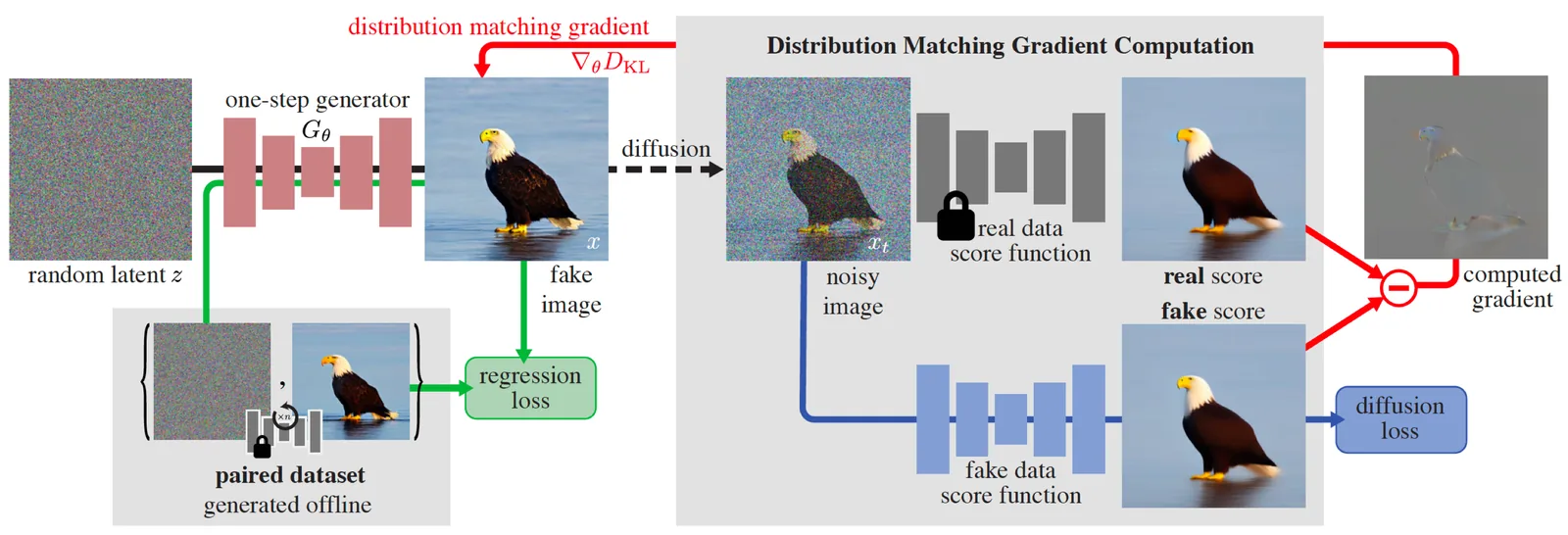
It distills a diffusion model into a one-step generator by matching distributions, not trajectories — the signal is a difference of two scores.
-
One-step generator (§3.1). The teacher predicts a clean image from one noised to step of . Copy its weights, drop the time input and pin it at the noisiest step: . Untrained, it outputs a washed-out average, but already maps noise to image.
-
Distribution matching objective (Eq. 1). Match the two image distributions, not the teacher's noise→image mapping: . Reverse KL, so mode-seeking — a bill paid later. Ablated: 2.62 → 9.21.
-
The gradient is what trains (Eq. 2). Densities are intractable, the gradient is not — a difference of scores : . Borrowed from ProlificDreamer, which optimizes one output at a time; DMD optimizes a generator.
-
Diffusing before scoring (Eq. 3). Neither score exists where the two distributions miss each other, so the generator's output is re-noised on the teacher's own schedule, , at a random . This is why both scores below take as an argument.
-
Frozen real score (Eq. 4). The teacher, frozen and read as a score: — the prediction minus the input, scaled, because a trained denoiser is a score estimator. It never moves, so is whatever the teacher learned, whose ceiling is DMD's.
-
Learned fake score (Eq. 5–6). The same formula over a second copy , retrained continually on the generator's own output by plain denoising, tracking a distribution that moves as the generator learns. GAN-like, two nets chasing — but no discriminator, no minimax.
-
Gradient weighting (Eq. 8). Scales that gradient so its magnitude is comparable across noise levels, using the teacher's own error on the sample. It reads like a footnote and is worth ~1 FID: DreamFusion's and ProlificDreamer's weightings give 3.60 / 3.71 on CIFAR-10, against 2.66.
-
Regression loss (Eq. 9). LPIPS against noise–image pairs sampled from the teacher's ODE solver, at under 1% of the compute. Needed because a score ignores rescaling of : mode dropping is a fixed point, not an instability. Ablated: 2.62 → 5.61; DMD2 drops it.
-
Alternating update (Alg. 1). on , unpaired samples for the first and paired for the second; on denoising, one update each per step. Three networks resident at once — the memory limit the paper names, and which it suggests LoRA could one day relieve.
-
Classifier-free guidance (§3.4). The pairs and come from the guided teacher, is left alone; the scale is baked in, so no CFG knob.
-
Experiments (§4). ImageNet-64 and CIFAR-10 by FID, MS COCO-30K by FID and CLIP after distilling SD v1.5 on LAION-Aesthetics: one step reads 2.62 on ImageNet, within 0.3 of the 512-step EDM teacher, and 11.49 on COCO against SD's 8.78 — 0.09s an image, 30× faster.
-
The high-guidance model is the honest one (§4.3, Tab. 4). The COCO table runs at CFG 3, the scale that minimizes the teacher's FID; a second model distilled at scale 8 reads 14.93 against the teacher's 13.45, a narrower gap, and beats every 4-step solver and LCM-LoRA.
The algorithms and their code. DMD was never released, so this is
DMD2's edm_guidance.py, condensed — but the distribution-matching core is untouched:
is Algorithm 2 exactly.
DMD2's GAN loss and its 5:1 update rule both live elsewhere in the same file.
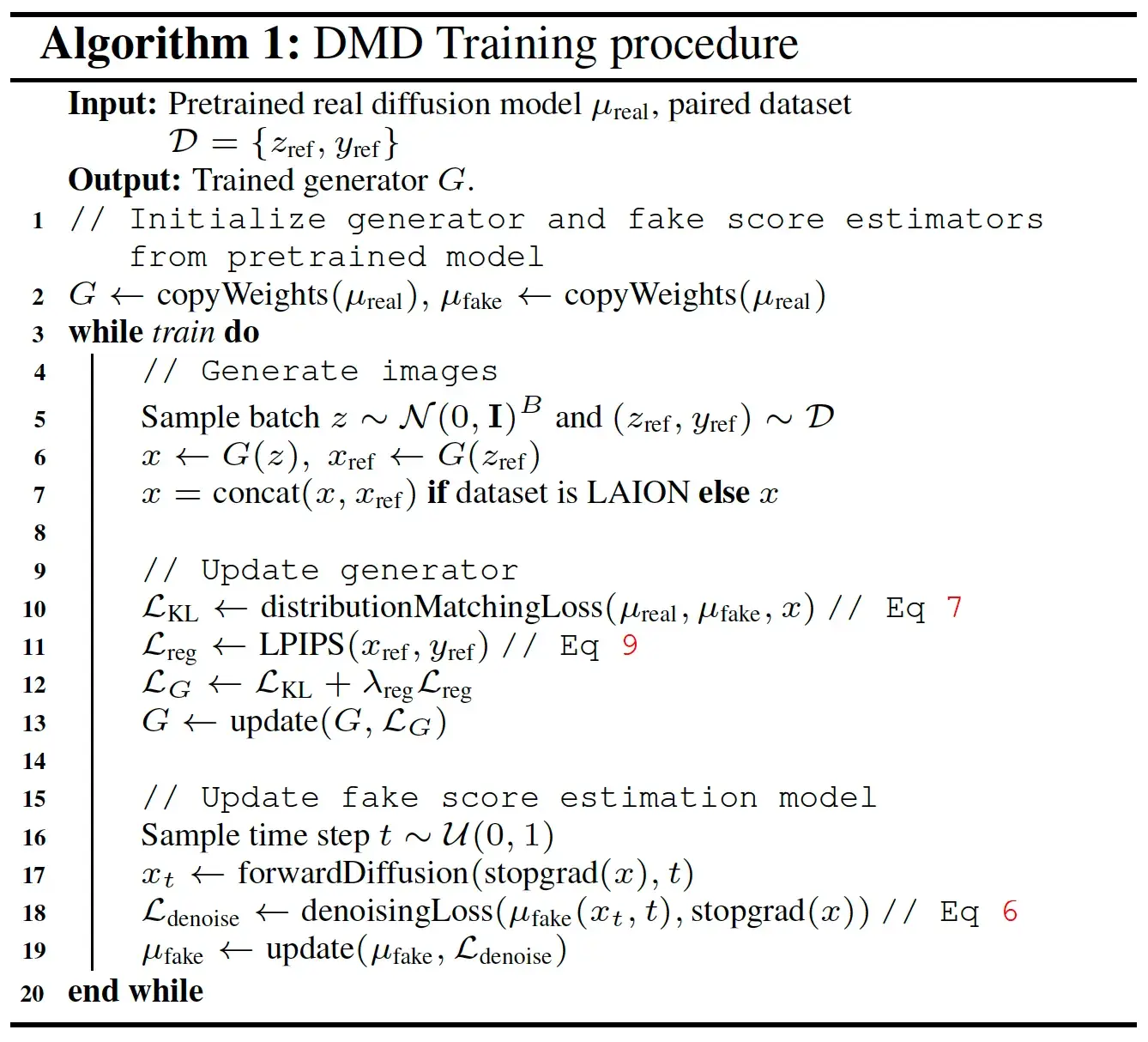
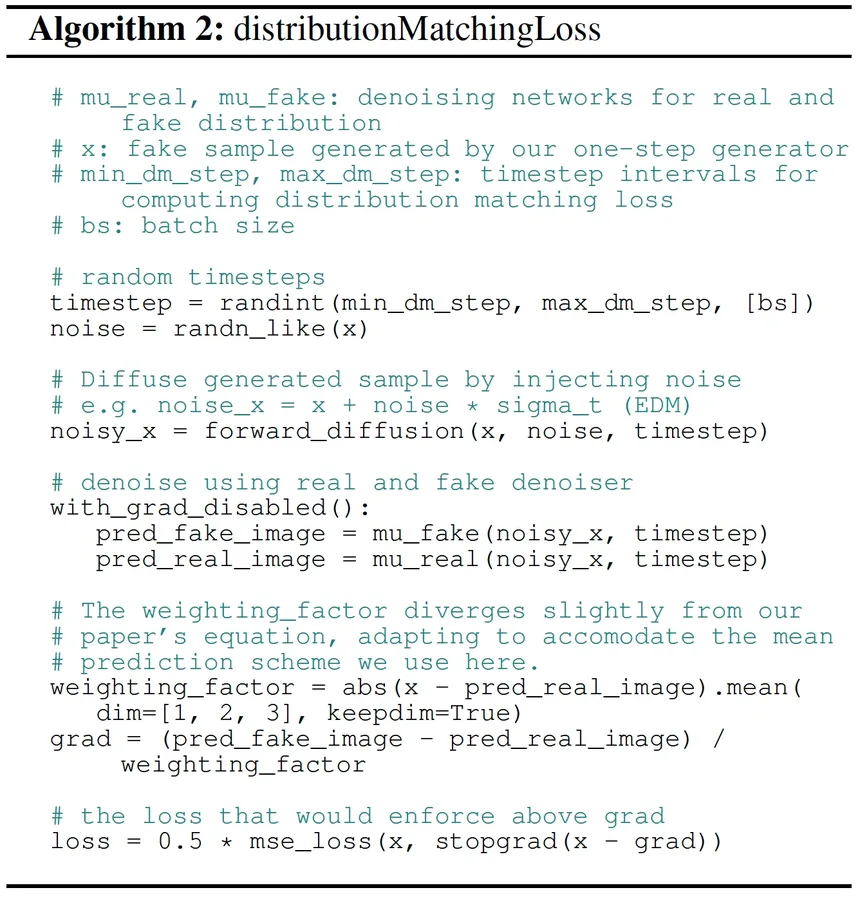
weighting_factor "diverges slightly" from Eq. 8, reading to suit a network that predicts the mean, not the noise.# Line 2: three copies of the teacher, two trainable.
generator = copy(real_unet) # G, one step
fake_unet = copy(real_unet) # mu_fake, Eq. 5
real_unet.requires_grad_(False) # mu_real, Eq. 4
min_step, max_step = int(0.02 * T), int(0.98 * T)
for _ in range(iters): # line 3
# Lines 5-7: one forward pass, no sampler loop.
z, (z_ref, y_ref) = randn(B, C, H, W), next(pairs)
latents, x_ref = generator(z), generator(z_ref)
if dataset == "laion":
latents = cat([latents, x_ref])
# Line 10 calls Alg. 2, inlined from here down.
with torch.no_grad():
t = randint(min_step, max_step + 1)
sigma = karras_sigmas[t]
noisy = latents + sigma * randn_like(latents)
# Eq. 4 is frozen; Eq. 5 is still learning.
p_real = latents - real_unet(noisy, sigma, labels)
p_fake = latents - fake_unet(noisy, sigma, labels)
# Eq. 8, and then the objective itself.
weight = p_real.abs().mean([1,2,3], keepdim=True)
grad = (p_real - p_fake) / weight
# A carrier, not a loss: differentiating it hands
# `grad` straight to the generator.
target = (latents - grad).detach()
loss_dm = 0.5 * F.mse_loss(latents, target)
# Lines 11-13.
loss = loss_dm + lambda_reg * lpips(x_ref, y_ref)
loss.backward(); opt_g.step(); opt_g.zero_grad()
# Lines 16-19: the fake score, refitted to the
# generator's own samples over the full range of t.
x = latents.detach() # no path back to G
sigma = karras_sigmas[randint(0, T)]
noisy = x + sigma * randn_like(x)
pred = fake_unet(noisy, sigma, labels)
w = snr + 1 / sigma_data**2 # Eq. 6
loss_fake = (w * (pred - x) ** 2).mean()
loss_fake.backward(); opt_fake.step()Adversarial Diffusion Distillation
Stability AI
European Conference on Computer Vision (ECCV), 2024
Nov 28, 2023 ADD (858) code (27.3K)
It first brought the adversarial loss into diffusion distillation — shipped as SDXL-Turbo — opening the GAN-assisted route that turbo-class generators still follow.
An adversarial loss keeps single-step samples sharp while score distillation keeps them faithful to the teacher — SDXL-Turbo, real time at one step.
-
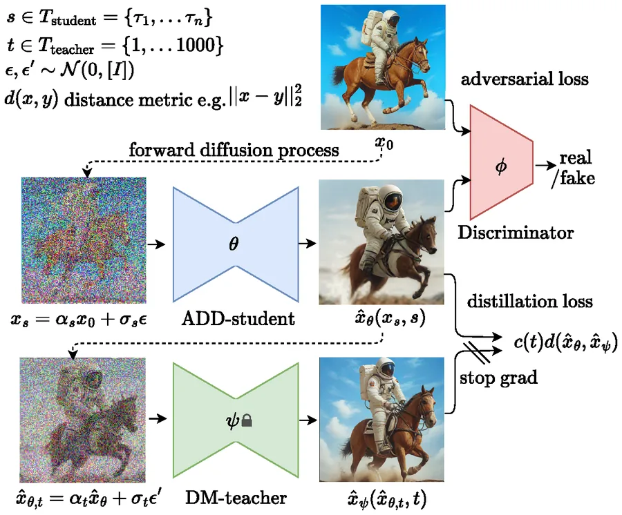
Three networks (§3.1). A student initialized from the pretrained UNet denoises at just timesteps with and zero terminal SNR, so the pure noise inference starts from stays in-distribution; a frozen teacher and a discriminator complete the training triangle (Fig. 1).
-
The adversarial half (§3.2). StyleGAN-T's recipe: frozen DINOv2 features, lightweight trainable heads, hinge loss with an R1 penalty on head inputs; the discriminator is projection-conditioned on the text — and, when , on the clean behind the student's noised input.
-
The distillation half (§3.3). The frozen teacher denoises a re-noised copy of the student's output — raw generations would be out-of-distribution for it — and the student regresses onto that under stopgrad: score distillation, computed in pixel space for the stabler gradients.
-
No guidance at inference (§3–4). CFG distills into the weights, cutting memory; one step beats LCM-XL and the single-step GANs, and at four steps ADD-XL outruns its own SDXL teacher in human preference — the first foundation-scale model running in real time at 512px.
-
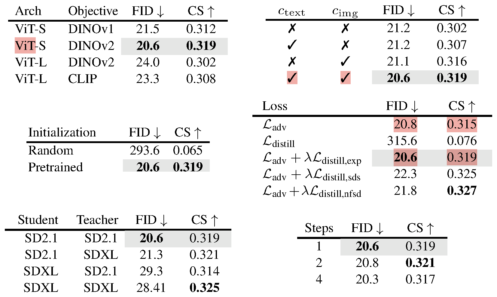
Experiments (§4). ADD-M (SD, 860M) and ADD-XL (SDXL, 3.1B) at 512px, COCO FID-5K and CLIP for ablations, ELO from raters for the ranking: ADD-M one step 19.7 / 0.326 against InstaFlow's 22.4 and 8-step DPM's 31.7; ADD-XL beats LCM-XL at one step and SDXL at four.
-
The student inherits the teacher, not the size (Tab. 1e). SDXL student and teacher score 28.41 FID against SD2.1's 20.6 while CLIP rises 0.319 → 0.325: the student takes its teacher's traits, SDXL's being less diverse, higher quality; a random init collapses to 293.6 (1c).
On Distillation of Guided Diffusion Models
Stanford · Stability AI · Google Research, Brain Team
Conference on Computer Vision and Pattern Recognition (CVPR), 2023
Oct 06, 2022 CFG Distill (861)
It first made classifier-free guidance distillable by conditioning the student on the guidance scale — a -embedding now standard equipment in few-step generators.
It makes classifier-free guidance distillable — fold the two-model combination into a guidance-conditioned student, then progressively distill it.
-
Why guidance resists distillation (§2). Classifier-free guidance runs two networks per step and mixes their outputs, ; the scale is a quality–diversity knob for the user, so a student has to cover a full range of guidance strengths rather than any single point of it.
-
Stage 1 folds the pair into one network (§3.1). A student regresses onto the guided mix with , the scale entering via Fourier embedding, like timestep; weights start from the teacher's conditional half. Range-training is free — it matches fixed-scale students (Tab. 1).
-
Stage 2 is PD, carrying along (§3.2). The merged model then walks progressive distillation's ladder unchanged — halve, re-teach, repeat — with v-prediction throughout. On pixel-space ImageNet-64 it matches its 1024x2-step teacher at 8–16 steps, a speedup of up to 256x.
-
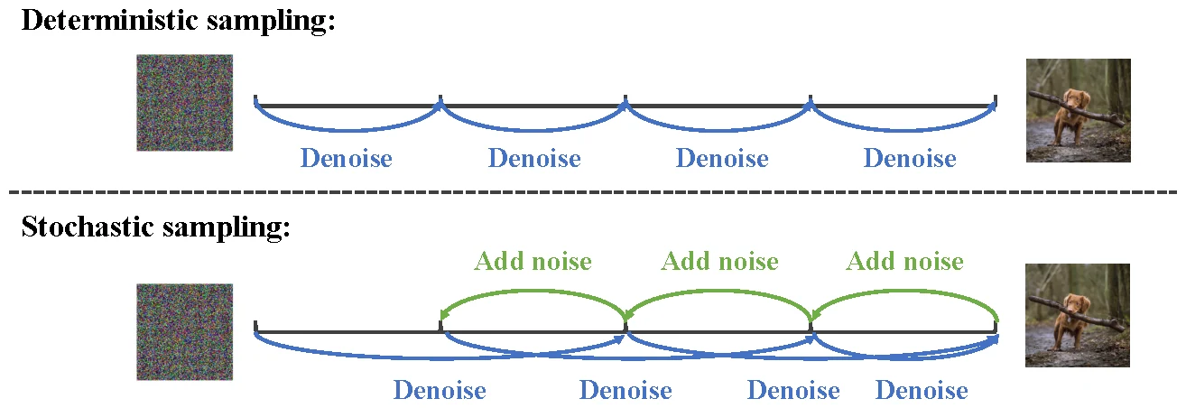
A stochastic sampler too (§3.3). One deterministic step at doubled length, then one re-noising step backward — the first study of distilling for samplers beyond deterministic DDIM, and it runs neck and neck with the deterministic variant across guidance scales (Tab. 1).
-
Experiments (§4). Pixel-space ImageNet-64 by FID / IS over , latent ImageNet-256, LAION-512, SDEdit and inpainting: ImageNet-64 at reads 2.17 at 4 steps against the teacher's 2.36 at 1024×2; LAION-512 37.3 / 26.0 at 2 / 4 steps against DPM++'s 98.8 / 34.1.
-
Metrics stop seeing it at 8 steps (§4.2.2, Fig. 7, 10). On 5000 COCO captions the distilled SD beats DDIM on FID and CLIP at 2 and 4 steps and ties at 8, while 8-step DDIM samples stay blurrier than 4 distilled ones — the paper's own admission that both metrics miss it here.
Progressive Distillation for Fast Sampling of Diffusion Models
Google Research, Brain Team
International Conference on Learning Representations (ICLR), 2022
Feb 01, 2022 PD (2,833) code
It opened the progressive route to few-step diffusion sampling, and its velocity parameterization outgrew distillation to become a standard for training diffusion models.
It halves a sampler's steps by distillation, over and over — 8192 down to 4 — introducing velocity prediction to keep few-step models stable.
-
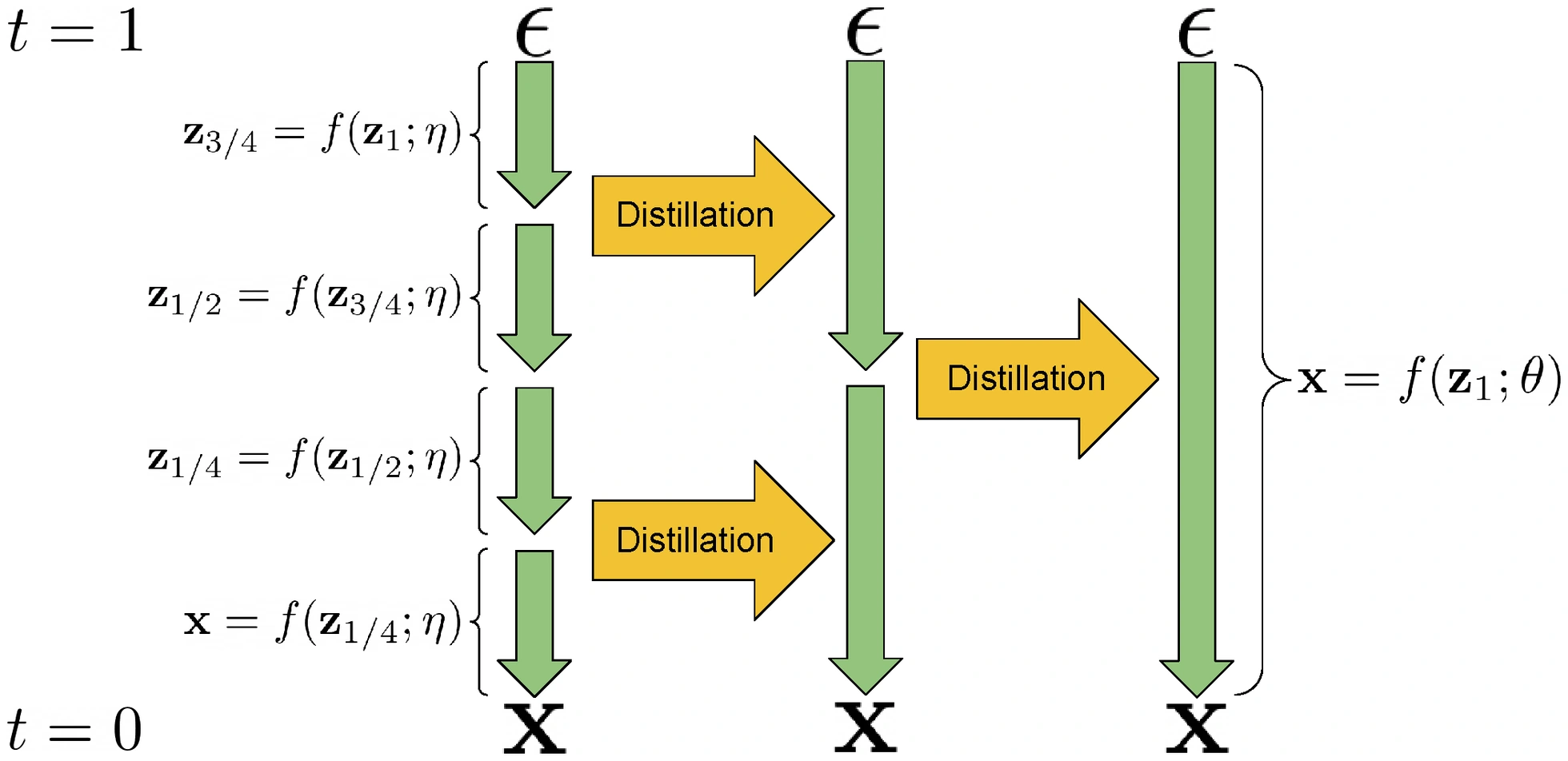
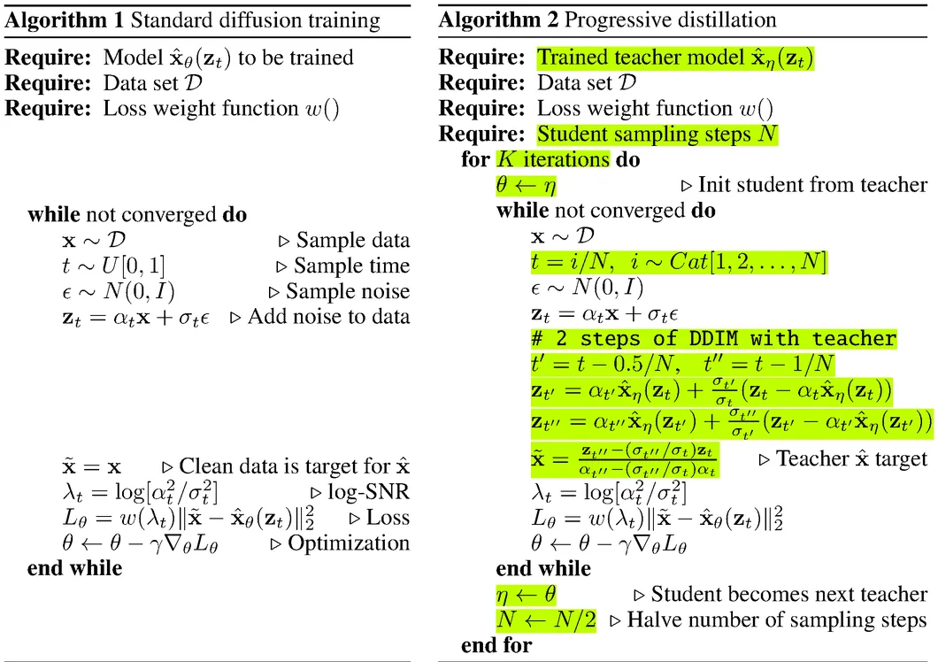
One student step = two teacher steps (§3, Alg. 2). The student starts as a copy of the teacher and trains like a normal diffusion model except for the target: from , run two teacher DDIM steps, then invert one student DDIM step to get the that reaches the same point in a single jump.
-
Why the target beats real data (§3). Given the real is ambiguous — many images produce the same noisy input, so standard training regresses to a blurry average. The target is fully determined by teacher and : sharp, which lets one step do two steps' work.
-
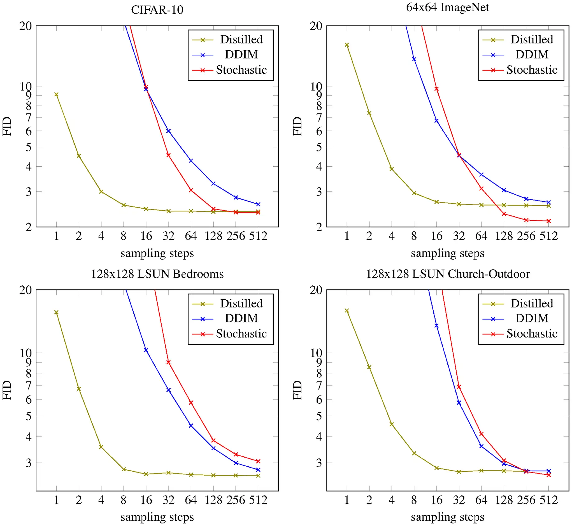
The halving ladder (§3). When the student converges it becomes the next teacher and halves: CIFAR-10 descends 8192 to 4 at 50K updates per rung, no more than the original training cost. FID holds near-optimal to 4–8 steps — 3.00 at 4 — where DDIM needs 50 for 4.67.
-
Where noise prediction breaks (§4). Distillation pushes evaluation toward zero SNR, where divides by a vanishing ; at one step the input is pure noise, so is the input and says nothing about — and the implicit SNR loss weighting gives that regime zero weight.
-
Velocity prediction (§4, App. D). Of three stable fixes — predict ; predict and jointly; predict — the last is stablest: on the angle , a DDIM update becomes a rotation whose step size ignores SNR. New weightings ride along: truncated SNR, SNR+1.
-
Against one-shot distillation (§6). Luhman & Luhman regress a one-step student on precomputed full-length teacher runs — a cost linear in the teacher's steps. PD never runs the teacher at full length — cost logarithmic — and hits 9.12 at one step against their 9.36.
-
Experiments (§5.2). CIFAR-10, ImageNet-64, LSUN Bedroom and Church, from 8192 or 1024 steps, FID after every halving against DDIM and a stochastic sampler: near-optimal to 4–8 steps on all four, sharp loss only at 1–2; CIFAR-10 2.57 / 3.00 / 4.51 / 9.12 at 8 / 4 / 2 / 1 steps.
-
Parameterization matters less than stability (§5.1, Tab. 1). From scratch on CIFAR-10, every stable choice lands within ~0.1 FID of the rest, and -prediction edges , 2.51 against 2.75 with DDIM; is chosen for the SNR-free step size, and with truncated SNR diverges.
One rung of the ladder, straight from the repo, cut to the lines that carry the idea:
# One stage (dpm.py, training_losses): the student trains on real data, not synthetic pairs.
i = randint(0, N)  # N = this stage's step count; distillation forces discrete times
logsnr_t, logsnr_mid, logsnr_s = sched((i+1) / N), sched((i+.5) / N), sched(i / N)  # cosine
z_t = alpha(logsnr_t) * x + sigma(logsnr_t) * randn_like(x)  # forward-noise a real image

# The target (Alg. 2): two teacher DDIM steps, then the x one student step must hit.
x1, eps1 = teacher(z_t, logsnr_t)  # every call yields x and eps views of one output
z_mid = alpha(logsnr_mid) * x1 + sigma(logsnr_mid) * eps1
x2, eps2 = teacher(z_mid, logsnr_mid)
z_s = alpha(logsnr_s) * x2 + sigma(logsnr_s) * eps2
frac = sigma(logsnr_s) / sigma(logsnr_t)
x_target = (z_s - frac * z_t) / (alpha(logsnr_s) - frac * alpha(logsnr_t))  # never clipped
x_target = where(i == 0, x1, x_target)  # bottom rung: the teacher's own prediction

# The loss (§4): v-parameterized student, truncated-SNR weighting.
v_pred = student(z_t, logsnr_t)  # student starts as a weight copy of the teacher
x_pred = alpha(logsnr_t) * z_t - sigma(logsnr_t) * v_pred
x_mse = mse(x_pred, x_target)
loss = max(x_mse, snr(logsnr_t) * x_mse)  # the paper's max(1, SNR), spelled max(x_mse, eps_mse)
# On convergence: teacher = student, N //= 2 - rerunning this file log2(N) times is the ladder.
Knowledge Distillation in Iterative Generative Models for Improved Sampling Speed
arXiv, 2021
Jan 07, 2021 Denoising Student (405) code (30)
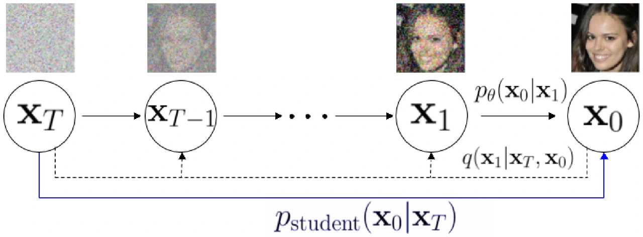
It distills a 100-step DDIM into a single forward pass by plain regression on the teacher's outputs, with no adversarial training anywhere.
-
A deterministic teacher is the precondition (§2). Distillation learns a function, and MCMC sampling is not one. Every DDIM step is fixed by its input, so the whole walk collapses into one function one network can learn — 100x faster than the teacher, 1000x than DDPM.
-
A KL that collapses to regression (§3.1, Eq. 10–11). Minimize between teacher and student conditionals ; both unit-variance Gaussians, so up to a constant it equals , their maps' outputs — MSE, no adversary, no joint training.
-
Training data is synthesized (§3.1). Draw from the prior, run the teacher (100 DDIM steps, 50 for LSUN), keep the pair — 1.024M per dataset, recycled over epochs. Every pair costs one full teacher run, so building the dataset scales linearly with the teacher's step count.
-
The student is the teacher, reused (§3.2). All the teacher's knowledge lives in one repeatedly applied network, so the student copies its architecture and weights, keeps predicting noise (subtracted from to form the sample), and is conditioned at the fixed top timestep .
-
What pixel-level replication costs (§4.1). The student must match the teacher's output down to the pixel, so unresolved detail averages to blur — 256px LSUN turns soft — and CIFAR-10's one-step 9.36 trails the 100-step teacher's 4.16, a gap distribution matching later closed.
-
Experiments (§4). CIFAR-10, CelebA-64 and LSUN Bedroom / Church by FID and IS against GANs, VAEs and EBMs: 9.36 / 8.36 on CIFAR-10, below NVAE's 51.67, far from StyleGAN2-ADA's 2.92; 10.68 on CelebA; 50K CIFAR samples in 51.5s against the teacher's 4,960s.
-
The latent survives distillation (§4.2). Spherical interpolation between two yields plausible morphs, and resizing the latent gives coherent images of a size never trained on — the student inherits the teacher's noise-to-image map and its generalization, not its samples.
The method straight from the repo, cut to the lines that carry the idea:
# Data (create_dataset.py): one (x_T, x_0) pair costs one full teacher run.
x = x_T = randn(B, res, res, 3)  # start from the prior
for i, j in zip(reversed(seq), reversed([-1, *seq[:-1]])):  # 100 steps quadratic; LSUN: 50 linear
    eps = teacher_unet(x, i)  # frozen pretrained DDPM/DDIM weights
    x = sqrt(a[j]) * (x - sqrt(1 - a[i]) * eps) / sqrt(a[i]) + sqrt(1 - a[j]) * eps  # eta = 0; a[-1] = 1
pairs.save(fp16(x_T), uint8(x))  # 1.024M pairs, built once, recycled every epoch

# Student (models.py): the teacher reused, pinned to the top timestep.
def student(z):
    eps = teacher_unet(z, t=999)  # same net, same weights, t fixed at T
    return z - eps  # still reads as noise prediction; one subtraction ends sampling

# Loss (training.py): Eq. 11 as plain regression on the synthesized pairs.
loss = sum((x_0 - student(x_T)) ** 2) / B  # CIFAR-10 actually ships |.| here - L1, not L2
Last updated on September 17, 2026 · Citations from Semantic Scholar & Google Scholar; stars from GitHub, September 2026