Architectures & Paradigms

Recast MeanFlow's self-written target as plain velocity regression, and turn its frozen guidance scale into one more test-time condition.

• What MeanFlow regresses (§3, Eq. 4–7). MeanFlow identity $u=v-(t-r)du/dt$ (Eq. 4), with $du/dt=v{\partial }_{z}u+{\partial }_{t}u\triangleq \mathrm{J}\mathrm{V}\mathrm{P}(u;v)$ (Eq. 5), makes $u$ trainable: target $u_{\mathrm{t}\mathrm{g}\mathrm{t}}=(e-x)-(t-r)\mathrm{J}\mathrm{V}\mathrm{P}(u_{\theta };e-x)$ (Eq. 6) is fitted by $𝔼\Vert u_{\theta }-\mathrm{s}\mathrm{g}(u_{\mathrm{t}\mathrm{g}\mathrm{t}}){\Vert }^2$ (Eq. 7) — $e-x$ standing for $v$ in both places.

• The identity read backwards (§4.1, Eq. 8–10). Solve for $v(z_t)=u(z_t)+(t-r)du/dt$ (Eq. 8), make it as $V_{\theta }\triangleq u_{\theta }+(t-r){\mathrm{J}\mathrm{V}\mathrm{P}}_{\mathrm{s}\mathrm{g}}(u_{\theta };e-x)$ (Eq. 9) and minimize $𝔼\Vert V_{\theta }-(e-x){\Vert }^2$ (Eq. 10) — fully equivalent to Eq. 6–7, and now a v-loss re-parameterized by u-pred.

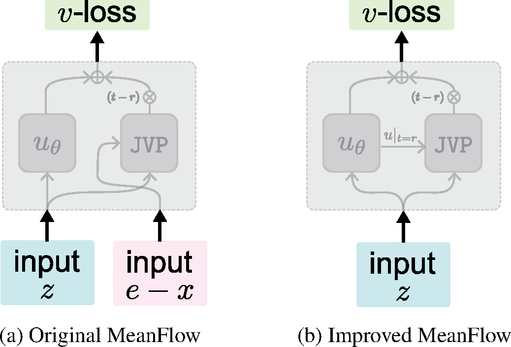
• The input that should not be there (Eq. 11, Fig. 1a). Written out, that compound function is $V_{\theta }(z_t,e-x)$, reading the conditional velocity as a second argument — illegitimate for a regressor of $z_t$, and traceable to Eq. 6, which put the conditional where Eq. 5 asks for the marginal.

• Predict the tangent instead (Eq. 12). $V_{\theta }(z_t)\triangleq u_{\theta }(z_t)+(t-r){\mathrm{J}\mathrm{V}\mathrm{P}}_{\mathrm{s}\mathrm{g}}(u_{\theta };v_{\theta })$ (Eq. 12) — both arguments are now network outputs of $z_t$ alone. Stop-gradient survives, but inside the prediction rather than on the target, and is kept because dropping it brings second-order gradients in $\theta$.

• Two cheap $v_{\theta }$ (§4.1, Tab. 1a). The boundary condition $v_{\theta }(z_t,t)\equiv u_{\theta }(z_t,t,t)$ is free — FID 32.69 → 29.42 unguided, 3.43 → 2.99 on XL/2. An auxiliary $v$-head over the last 8 layers, on its own flow-matching loss, free at inference, does worse unguided, 30.76, and better guided, 5.68.

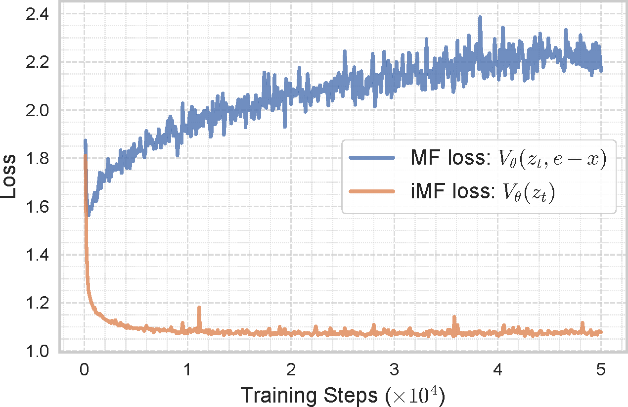
• Why the conditional tangent hurts (§4.1, Eq. 2, Fig. 3). Feeding $e-x$ to the loss leaks nothing, since the true regression target is the marginal $v(z_t)\triangleq 𝔼[e-x\mid z_t]$; but as the JVP's tangent its variance is magnified by the Jacobian it multiplies, which is what the two loss curves separate.

• Guidance, fixed and unfixed (§4.2, Eq. 13–15). MeanFlow bakes $v^{\mathrm{c}\mathrm{f}\mathrm{g}}(z_t\mid c)=\omega v(z_t\mid c)+(1-\omega )v(z_t)$ (Eq. 13) in at one $\omega$ chosen before training. iMF makes it an input, $V_{\theta }(·\mid c,\omega )\triangleq u_{\theta }(z_t\mid c,\omega )+(t-r){\mathrm{J}\mathrm{V}\mathrm{P}}_{\mathrm{s}\mathrm{g}}$ (Eq. 15), with $\omega ~p(\omega )\propto {\omega }^{-\beta }$ drawn on $[1,8]$, skewed toward the small $\omega$.

• The target it fits (App. A, Eq. 17). $v_{\mathrm{t}\mathrm{g}\mathrm{t}}=(e-x)+(1-1/\omega )(u_{\theta }(z_t\mid t,t,c)-u_{\theta }(z_t\mid t,t,\varnothing ))$ (Eq. 17) is MeanFlow's guided target with $\omega$ an input, so $\omega =1$ means no guidance. FID 5.68 → 5.52, small only because MeanFlow's fixed $\omega$ already suited the B/2 model.

• The interval is a condition too (§4.2, Tab. 1b). Pass $\Omega =\{\omega ,t_{min},t_{max}\}$, sampling $t_{min}~U[0,0.5]$ and $t_{max}~U[0.5,1]$ and switching guidance off ($\omega =1$) when $t$ falls outside — 5.52 → 4.57, while the $\omega =1$ column itself improves 30.76 → 20.95, so training across scales generalizes better.

• In-context conditioning (§4.3, Eq. 16, Tab. 1c). $u_{\theta }=u_{\theta }(z_t\mid r,t,c,\Omega )$ (Eq. 16) is too heterogeneous for one adaLN-zero to sum; replicate each into tokens — 8 for the class, 4 for the rest — concatenated with the image patches: 4.57 → 4.09, and 133M → 89M once adaLN is gone.

• Experiments (§5). ImageNet-256 in the VAE latent, from scratch, 1-NFE FID-50K on MeanFlow's code and B/2 baseline: the changes step 6.17 → 5.68 → 4.57 → 4.09, SwiGLU, RMSNorm and RoPE 3.82, 640 epochs 3.39 at 89M; iMF-XL/2 takes 1.72 at 1-NFE and 1.54 at 2-NFE.

• The size labels do not calibrate (§5.2, Tab. 2). Without adaLN-zero, parameters go to depth: iMF-XL/2 has 48 layers, 610M and 174.6 Gflops to MF-XL/2's 28, 676M and 119.0, so 1.72 against 3.43 is not at matched FLOPs; iMF-M/2's 2.27 at 49.9 Gflops over MF's 5.01 at 54.0 is.

The training and sampling algorithm and its code. Follow Algorithm 2 of paper.

def train():
  # 1. Sample timesteps r and t from lognorm(-0.4, 1.0), sorted so r <= t; 50% of rows get r = t
  r, t = sample_time_steps(bs)

  # 2. Sample the guidance scale and interval; rows with r = t get the full interval [0, 1]
  omega = sample_cfg_scale(bs)  # omega ~ omega^-beta on [1, 8]; assume beta=1
  t_min, t_max = sample_cfg_interval(bs, r == t)  # t_min ~ U[0, 0.5], t_max ~ U[0.5, 1]

  # 3. Build the noisy latent z_t and its velocity v_t
  z_t = (1 - t) * z_0 + t * noise  # linear path
  v_t = noise - z_0  # conditional velocity

  # 4. Predict the average velocity u and the instantaneous velocity v with a class dropout
  dropped = rand(bs) < 0.1  # 10% class dropout
  y_in = where(dropped, null, y)
  u, v = model(z_t, r, t, omega, t_min, t_max, y=y_in)  # Eq. (16); omega and the interval are inputs

  # 5. Predict cond and uncond instantaneous velocity at t with the v head; omega = 1 outside the interval
  omega_t = where((t >= t_min) & (t <= t_max), omega, 1)
  with no_grad():
      v_c, v_u = model(cat([z_t, z_t]), cat([t, t]), cat([t, t]), cat([omega_t, ones]), cat([zeros, zeros]),
                       cat([ones, ones]), y=cat([y, null]), predict_u=False).chunk(2)

  # 6. Build the guided velocity target
  v_target = v_t + (1 - 1 / omega_t) * (v_c - v_u)  # Eq. (17)
  v_target = where(dropped, v_t, v_target)

  # 7. Build the compound prediction V, with the predicted v_c as the JVP tangent
  fn = lambda z, r_, t_: model(z, r_, t_, omega, t_min, t_max, y=y_in, predict_v=False)
  _, dudt = jvp(fn, (z_t, r, t), (v_c, zeros_like(r), ones_like(t)))  # no_grad, so dudt is sg(du/dt)
  V = u + (t - r) * dudt  # Eq. (15)

  # 8. Calculate loss of the u head and the auxiliary v head
  loss = adaptive_loss(V - v_target) + adaptive_loss(v - v_target)  # sum of squared error / (sg(.) + 0.01)^1
  loss = loss.mean()


def sample():
  time_steps = linspace(1, 0, num_steps + 1)
  for i in range(num_steps):
      t = full((bs,), time_steps[i])
      r = full((bs,), time_steps[i + 1])
      u, _ = model(z, r, t, omega, t_min, t_max, y=y, predict_v=False)  # guidance is a condition: one forward
      z = z - (t - r) * u

Model the average velocity over an interval instead of the instantaneous one — a one-step generator trained from scratch, with guidance in the field.

• Average velocity (§4.1, Eq. 3). $u(z_t,r,t)\triangleq (1/(t-r)){\int }_r^{t}v(z_{\tau },\tau )d\tau$ — displacement across $[r,t]$, a field induced by $v$ itself and by no network; ${lim}_{r\to t}u=v$, and integral additivity already gives $(t-r)u(z_t,r,t)=(s-r)u(z_s,r,s)+(t-s)u(z_t,s,t)$, consistency with nothing imposed.

• The MeanFlow identity (Eq. 6). Multiply the definition by $t-r$ and differentiate in $t$ with $r$ fixed; the product rule and the fundamental theorem give $u+(t-r)du/dt=v$, that is $u(z_t,r,t)=v(z_t,t)-(t-r)du/dt$ — the intractable integral traded for a local relation between the fields.

• One JVP computes it (Eq. 8, Tab. 1b). $du/dt=(d{z}_t/dt){\partial }_{z}u+(dr/dt){\partial }_{r}u+(dt/dt){\partial }_{t}u=v{\partial }_{z}u+{\partial }_{t}u$, since $d{z}_t/dt=v$, $dr/dt=0$: a Jacobian–vector product with tangent $(v,0,1)$, one extra backward pass. Corrupt it and one-step collapses — 61.06 FID against 137.96–329.22.

• The objective (Eq. 9–11). $ℒ(\theta )=𝔼\Vert u_{\theta }(z_t,r,t)-\mathrm{s}\mathrm{g}(u_{\text{tgt}}){\Vert }_2^2$ with $u_{\text{tgt}}=v_t-(t-r)(v_t{\partial }_z{u}_{\theta }+{\partial }_t{u}_{\theta })$: the network's own partials stand in for those of the true $u$, the conditional $v_t$ for the marginal, and stop-gradient removes double backpropagation. Zero loss recovers the identity, hence Eq. 3.

• Sampling (§4.1, Eq. 12). $z_r=z_t-(t-r)u_{\theta }(z_t,r,t)$ — the integral is the prediction, so $z_0=z_1-u_{\theta }(z_1,0,1)$ is one call, few steps chaining it.

• Guidance inside the field (§4.2, Eq. 19). Define $v^{\text{cfg}}\triangleq \omega v(z_t,t\mid c)+(1-\omega )v(z_t,t)$ and average it; since $v^{\text{cfg}}(z_t,t)=v(z_t,t)=u^{\text{cfg}}(z_t,t,t)$, the unconditional half is the network's own diagonal, ${\tilde{v}}_t=\omega v_t+(1-\omega )u_{\theta }(z_t,t,t)$, so guidance stays a single call ($\omega =3$ gives 15.53).

• Guidance, improved (App. B.1, Eq. 21, Tab. 5). A mixing scale $\kappa$ lets the class-conditional diagonal into the target as well: ${\tilde{v}}_t\triangleq \omega (ϵ-x)+\kappa u_{\theta }(z_t,t,t\mid c)+(1-\omega -\kappa )u_{\theta }(z_t,t,t)$; solving it gives Eq. 13's form $v^{\text{cfg}}(z_t,t\mid c)={\omega }^{\prime }v(z_t,t\mid c)+(1-{\omega }^{\prime })v(z_t,t)$ at the effective scale ${\omega }^{\prime }=\omega /(1-\kappa )$. At a fixed ${\omega }^{\prime }=2$, $\kappa$ from 0 to 0.9 takes the 1-NFE FID 20.15 → 18.63; the released XL/2 ships $\omega =1$, $\kappa =0.5$.

• Adaptive loss weighting (§4.3, App. B.2, Tab. 1e). For the error $\Delta =u_{\theta }-u_{\text{tgt}}$, the powered loss $\Vert \Delta {\Vert }_2^{2\gamma }$ equals the squared $L_2$ loss under the weight $w=1/(\Vert \Delta {\Vert }_2^2+c{)}^p$, $p=1-\gamma$, $c={10}^{-3}$, applied as $\mathrm{s}\mathrm{g}(w)·\Vert \Delta {\Vert }_2^2$: $p=1$ gives 61.06, Pseudo-Huber-like $p=0.5$ 63.98, plain $L_2$ 79.75.

• Two clocks (§4.3, Tab. 1a/c/d). $(r,t)$ come from lognorm$(-0.4,1.0)$, and $t>r$, and only 25% of pairs keep $r\ne t$ — at 0% the correction vanishes, the loss is exactly flow matching and 1-NFE fails (328.91 against 61.06). The network is fed $(t,t-r)$, best of four embeddings.

• Experiments (§5). ImageNet-256 in a VAE latent, FID-50K at 1-NFE, plus CIFAR-10: B/2 to XL/2 reads 6.17 / 5.01 / 3.84 / 3.43 at 240 epochs (Shortcut 10.60), 2.20 at 2-NFE trained longer, DiT-XL/2's 2.27 at 250×2; CIFAR-10 2.92 without EDM preconditioning, against iCT's 2.83.

The training and sampling algorithm and its code. Follow Algorithm 1 and 2 of paper.

def train():
  # 1. Sample timesteps r and t from lognorm(-0.4, 1.0), sorted so r <= t
  r, t = sample_time_steps(bs)

  # 2. Build the noisy latent z_t and its velocity v_t
  z_t = (1 - t) * z_0 + t * noise  # linear path
  v_t = noise - z_0  # conditional velocity

  # 3. Predict the average velocity u with a class dropout
  dropped = rand(bs) < 0.1  # 10% class dropout
  y = where(dropped, null, y)
  u = model(z_t, r, t, y)

  # 4. Build CFG-guided velocity
  with no_grad():
      u_c, u_u = model(cat([z_t, z_t]), cat([t, t]), cat([t, t]), y=cat([y, null])).chunk(2)
  v_tilde = 0.2 * v_t + 0.92 * u_c + (1 - 0.2 - 0.92) * u_u  # Eq. 21; assume omega=0.2, kappa=0.92
  v_hat = where((t <= 0.8) & ~dropped, v_tilde, v_t)

  # 5. Calculate average velocity target
  _, dudt = jvp(lambda z, r_, t_: model(z, r_, t_, y), (z_t, r, t), (v_hat, zeros_like(r), ones_like(t)))  # Eq. 8
  u_target = v_hat - (t - r) * dudt  # Eq. 10

  # 6. Calculate loss
  loss = (u - u_target.detach()).square().flatten(1).sum(1)  # Eq. 9
  loss = (loss / (loss.detach() + 0.01)).mean()  # p=1, c=0.01 as the official code; paper: c=1e-3


def sample():
  time_steps = linspace(1, 0, num_steps + 1)
  for i in range(num_steps):
      t = full((bs,), time_steps[i])
      r = full((bs,), time_steps[i + 1])
      z = z - (t - r) * model(z, r, t, y=y)

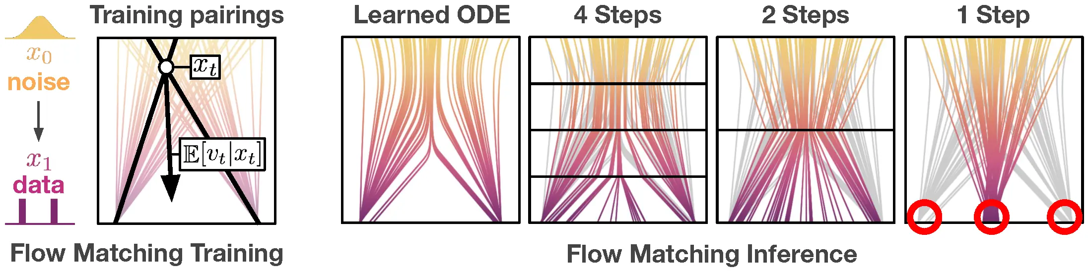
One network, conditioned on step size, jumps any distance along the flow — trained in one run, with no teacher, schedule, or second stage.

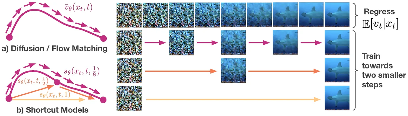
• Why naive one-step fails (§2, Fig. 2). Flow matching learns the average direction over all pairings passing through $x_t$; at $t=0$ that average points at the dataset mean, so one big Euler step lands there — multimodal data is unreachable in a single step even at the optimum.

• Condition on the step size (§3, Eq. 3). The shortcut is the normalized jump to the correct next point, $x_{t+d}^{\prime }=x_t+s(x_t,t,d)d$; at $d\to 0$ it is the flow itself, so shortcut models generalize flow matching — one model serves every budget from 128 steps to one.

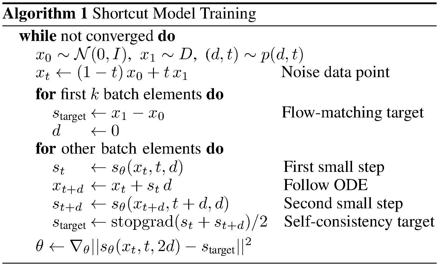
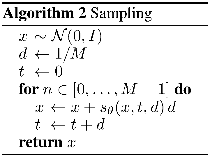
• Self-consistency instead of a teacher (§3, Eq. 4–5). One step equals two chained halves, $s(x_t,t,2d)=s(x_t,t,d)/2+s(x_{t+d}^{\prime },t+d,d)/2$: bootstrap targets come from the model itself, while a batch fraction at $d=0$ regresses flow matching. One run, ~16% extra compute.

• A binary grid of step sizes (§3.1). 128 base units give eight shortcut lengths $d\in (1/128,\dots ,1)$, each trained against two of the next size down, keeping bootstrap paths short; many-step quality matches the flow baseline, few- and one-step matches two-stage distillation methods.

• Experiments (§5). CelebA-HQ-256 and ImageNet-256, every objective retrained on one DiT-B codebase at matched compute, FID-50K at 128 / 4 / 1 steps: 6.9 / 13.8 / 20.5 and 15.5 / 28.3 / 40.3 — past every end-to-end and two-stage method but progressive distillation's one step.

• Bootstrapping still scales, and drives robots (§5.3–5.5). Unlike Q-learning, one-step FID keeps falling with size (DiT-XL: 10.6, 3.8 at 128 steps), and as a one-step policy on Push-T and Transport it scores 0.87 / 0.80 where a one-step diffusion policy collapses to 0.12 / 0.00.

The method straight from the repo, cut to the lines that carry the idea:

# One batch, two target kinds (targets_shortcut.py); 1/bootstrap_every of it bootstraps.
dt_base = ladder_index  # the network is conditioned on the log2 exponent, not on dt itself
dt = 1 / 2**dt_base  # the binary ladder [1, 1/2, ..., 1/128]
t = randint(0, 2**dt_base) / 2**dt_base  # t lands only on multiples of dt
x_t = (1 - (1 - 1e-5) * t) * x_0 + t * x_1  # a 1e-5 noise floor, not an exact lerp

# Bootstrap targets: two half-steps of the model itself (EMA and CFG both optional).
v1 = model(x_t, t, dt_base + 1)  # +1 = one rung down the ladder, step dt/2
x_mid = clip(x_t + (dt/2) * v1, -4, 4)  # clipped midpoint - stability the paper never mentions
v2 = model(x_mid, t + dt/2, dt_base + 1)
v_target = clip((v1 + v2) / 2, -4, 4)  # no grad flows through targets

# Flow-matching targets for the rest of the batch, on the finest grid.
t = randint(0, 128) / 128
v_target = x_1 - (1 - 1e-5) * x_0  # empirical velocity; dt_base = log2(128) encodes d = 0

# One loss serves both target kinds (train.py).
loss = mean((model(x_t, t, dt_base) - v_target) ** 2)

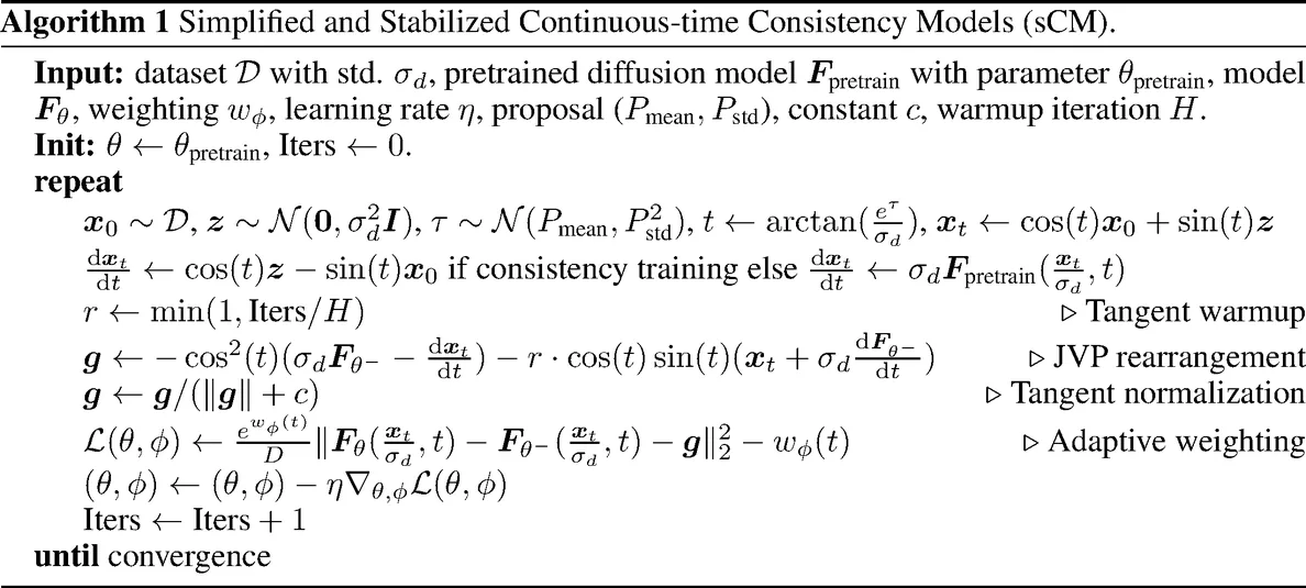
Simplify consistency models, stabilize the continuous-time limit by taming its tangent, scale to 1.5B: two steps within 10% of the teacher.

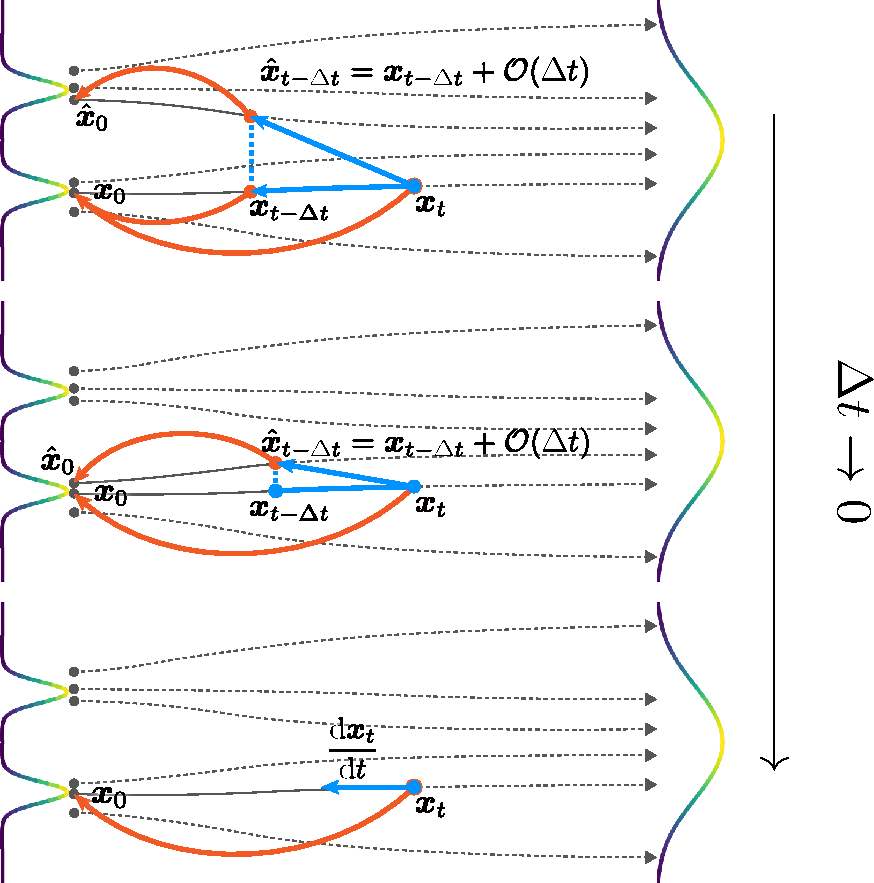
• The continuous-time limit (§2.2, Eq. 2). A consistency model $f_{\theta }(x_t,t)$ maps any trajectory point to its start, $f_{\theta }(x,0)\equiv x$. Discrete-time CMs match adjacent times, $𝔼[w(t)d(f_{\theta }(x_t,t),f_{{\theta }^{-}}(x_{t-\Delta t},t-\Delta t))]$, $x_{t-\Delta t}$ from an ODE solver: solver error plus a hand-tuned $\Delta t$ schedule. With ${\ell }_2$, as $\Delta t\to 0$ the gradient is ${\nabla }_{\theta }𝔼[w(t)f_{\theta }^{\top }d{f}_{{\theta }^{-}}/dt]$ with the tangent $d{f}_{{\theta }^{-}}/dt={\nabla }_{x_t}{f}_{{\theta }^{-}}d{x}_t/dt+{\partial }_t{f}_{{\theta }^{-}}$: solver-free, and until now unstable.

• TrigFlow (§3, Eq. 3–5). With noise $z~𝒩(0,{\sigma }_d^{2}I)$ at the data's scale, $x_t=\cos (t)x_0+\sin (t)z$, $t\in [0,\pi /2]$: EDM's coefficients become $c_{\text{skip}}=\cos (t)$, $c_{\text{out}}=-{\sigma }_d\sin (t)$, $c_{\text{in}}\equiv 1/{\sigma }_d$; the PF-ODE is $d{x}_t/dt={\sigma }_d{F}_{\theta }(x_t/{\sigma }_d,c_{\text{noise}}(t))$, trained on $\Vert {\sigma }_d{F}_{\theta }-v_t{\Vert }_2^2$ with $v_t=\cos (t)z-\sin (t)x_0$; the CM is a DDIM step, $f_{\theta }(x_t,t)=\cos (t)x_t-\sin (t){\sigma }_d{F}_{\theta }(x_t/{\sigma }_d,c_{\text{noise}}(t))$. EDM enters by $t=\arctan (\sigma /{\sigma }_d)$; flow matching is a special case.

• Where the tangent blows up (§4.1, Eq. 6–7). $d{f}_{{\theta }^{-}}/dt=-\cos (t)({\sigma }_d{F}_{{\theta }^{-}}-d{x}_t/dt)-\sin (t)(x_t+{\sigma }_{d}d{F}_{{\theta }^{-}}/dt)$: $F$, the ODE and $x_t$ are tame and ${\nabla }_{x_t}F·d{x}_t/dt$ well-conditioned, so the culprit is $\sin (t){\partial }_t{F}_{{\theta }^{-}}=\sin (t){\partial }_t{c}_{\text{noise}}·\partial \mathrm{e}\mathrm{m}\mathrm{b}/\partial c_{\text{noise}}·\partial F_{{\theta }^{-}}/\partial \mathrm{e}\mathrm{m}\mathrm{b}$ — three factors, one fix each. Fig. 4: EDM with Fourier scale 16 sends the norm past 150, positional EDM still explodes at $t\to \pi /2$, TrigFlow stays under 4, on CIFAR-10 models.

• Three architectural fixes (§4.1). (1) $c_{\text{noise}}(t)=t$: EDM's $\log ({\sigma }_d\tan t)$ gives $\sin (t){\partial }_t{c}_{\text{noise}}=1/\cos (t)\to \infty$. (2) Positional time embeddings: the derivative of $\mathrm{e}\mathrm{m}\mathrm{b}(c)=\sin (s·2\pi \omega c+\varphi )$ scales with $s$; positional means $s\approx 0.02$ — iCT's scale, explained. (3) Adaptive double normalization, $y=\mathrm{n}\mathrm{o}\mathrm{r}\mathrm{m}(x)\odot \mathrm{p}\mathrm{n}\mathrm{o}\mathrm{r}\mathrm{m}(s(t))+\mathrm{p}\mathrm{n}\mathrm{o}\mathrm{r}\mathrm{m}(b(t))$: raw AdaGN made CMs diverge; pixel-normalizing scale and shift keeps its expressivity.

• Tangent normalization (§4.2, Fig. 5a). Most gradient variance rides on $d{f}_{{\theta }^{-}}/dt$, so replace it by $g/(\Vert g\Vert +c)$, $c=0.1$, or clip it to $[-1,1]$: on ImageNet 512 either pulls 1-step FID well below the raw tangent's, and the two land together — applied before the weighting below.

• Adaptive weighting (§4.2, Eq. 8, App. D). The identity ${\nabla }_{\theta }𝔼[F_{\theta }^{\top }y]=\frac{1}{2}{\nabla }_{\theta }𝔼\Vert F_{\theta }-F_{{\theta }^{-}}+y{\Vert }_2^2$ turns Eq. 2 into an MSE, so EDM2's learned weight applies: ${ℒ}_{\text{sCM}}=𝔼[e^{w_{\varphi }(t)}/D\Vert F_{\theta }-F_{{\theta }^{-}}-\cos (t)d{f}_{{\theta }^{-}}/dt{\Vert }_2^2-w_{\varphi }(t)]$, the prior weight $1/({\sigma }_d\tan t)$ turning $\sin (t)$ into $\cos (t)$; at the optimum every time's weighted loss is 1. Times come from $t=\arctan (e^{\tau }/{\sigma }_d)$, $\tau ~𝒩(P_{\text{mean}},P_{\text{std}}^2)$ with $P_{\text{mean}}\le -0.8$: near clean data, where the real signal enters.

• Diffusion init and tangent warmup (§4.2, App. G). Init is the teacher's EMA; the $\sin (t)$ term is scaled by $r=min(1,\text{iters}/10\text{k})$, optional, against gradient spikes. Distillation costs ~2× a diffusion step and reaches the teacher's 2-step quality within ~20k iterations, under 20% of its compute.

• Discrete never catches up (§4.2, App. E, Fig. 5c). Every fix ports to discrete time through ${\Delta }_{{\theta }^{-}}(x_t,t,t^{\prime })=(f_{{\theta }^{-}}(x_t,t)-f_{{\theta }^{-}}(x_{t^{\prime }},t^{\prime }))/\sin (t-t^{\prime })$, $x_{t^{\prime }}$ one DDIM step away, which tends to $d{f}_{{\theta }^{-}}/dt$ as $t^{\prime }\to t$ (Eq. 37) and replaces the JVP in Eq. 8 unchanged; on $N$ EDM-spaced levels ($\rho =7$), FID improves with $N$ up to 1024, worsens past it from numerical precision, and on ImageNet 512 the continuous model sits below every $N$.

• JVP rearrangement (§5.1). The tangent $d{F}_{{\theta }^{-}}/dt={\nabla }_{x_t}{F}_{{\theta }^{-}}·d{x}_t/dt+{\partial }_t{F}_{{\theta }^{-}}$ overflows in FP16 near $t=0$ and $\pi /2$. The loss needs only $\cos (t)df/dt\propto \cos (t)\sin (t)dF/dt$, so the JVP is fed the tangent $(\cos (t)\sin (t)d{x}_t/dt,\cos (t)\sin (t){\sigma }_d)$ at $(x_t/{\sigma }_d,t)$ — the scale folded in upstream.

• Flash-attention JVP (§5.1, App. F). For $y=\mathrm{s}\mathrm{o}\mathrm{f}\mathrm{t}\mathrm{m}\mathrm{a}\mathrm{x}(x)V=pV$ the output tangent is $t_y=p{t}_V+(p\odot t_x)V-(p{t}_x^{\top })y$; the two new terms need only a running vector $g=(e^{x-m}\odot t_x)V$ and scalar $\mu ={\sum }_i{e}^{x_i-m}{t}_{x,i}$, merged block by block like Flash Attention's own $m,\ell ,f$ — $g$ rescaled by $e^{m_a-m}$, $\mu$ summed the same way — and read out as $t_{p}V=g/\ell -(\mu /\ell )y$, so attention and its JVP come out of one pass with no attention matrix stored.

• Sampling and guidance (§5.2, App. G). One step from $t_{max}=\arctan (80/{\sigma }_d)$, two steps re-noising to $t=1.1$. On ImageNet 512 CFG is distilled in: the student takes the guidance scale $s~𝒰[1,2]$ as an input embedded like $t$, the teacher at that scale; sCT, teacher-free, gets none.

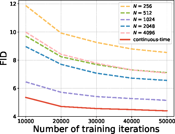
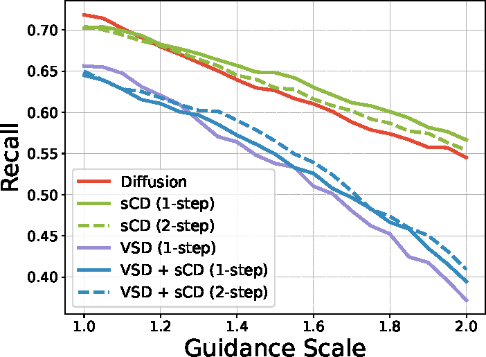
• Experiments (§5.2, Tab. 1–2). CIFAR-10, ImageNet 64 and 512, FID at 1 / 2 steps for sCT and sCD: two steps already read 2.06 / 1.48 / 1.88 against teachers 2.01 / 1.33 / 1.73; 1-step sCD-XXL 2.28 beats StyleGAN-XL's 2.41 and VAR's 2.63 at under 10% of their compute.

• sCD scales like its teacher; sCT does not in latent space (Fig. 6, Tab. 2). The sCD/teacher FID ratio holds at ~1.3 (one step) and ~1.09 (two) from S to XXL, so the gap shrinks; sCT wins at 64px but reads 10.13 against sCD's 3.07 at 512-S, variance blamed on the VAE latent.

• VSD buys precision with recall; sCD keeps both (Fig. 7, Tab. 7). From guidance 1 to 2 VSD's recall collapses as under heavy guidance, as 2-step sCD tracks the teacher; VSD on top of sCD moves 1-step FID only 2.75 → 2.67 but FD-DINOv2 83.78 → 54.81: the metrics disagree.

Consistency training grown up — drop the teacher-side EMA, swap LPIPS for Pseudo-Huber, grow the discretization, and beat distillation.

• Why leave CD and LPIPS (§1). Distillation caps a student at its teacher; LPIPS leaks ImageNet features into FID, whose Inception judge saw the same data. iCT drops both and wins anyway: one-step FID 2.51 on CIFAR-10 and 3.25 on ImageNet-64, past CD at one and two steps.

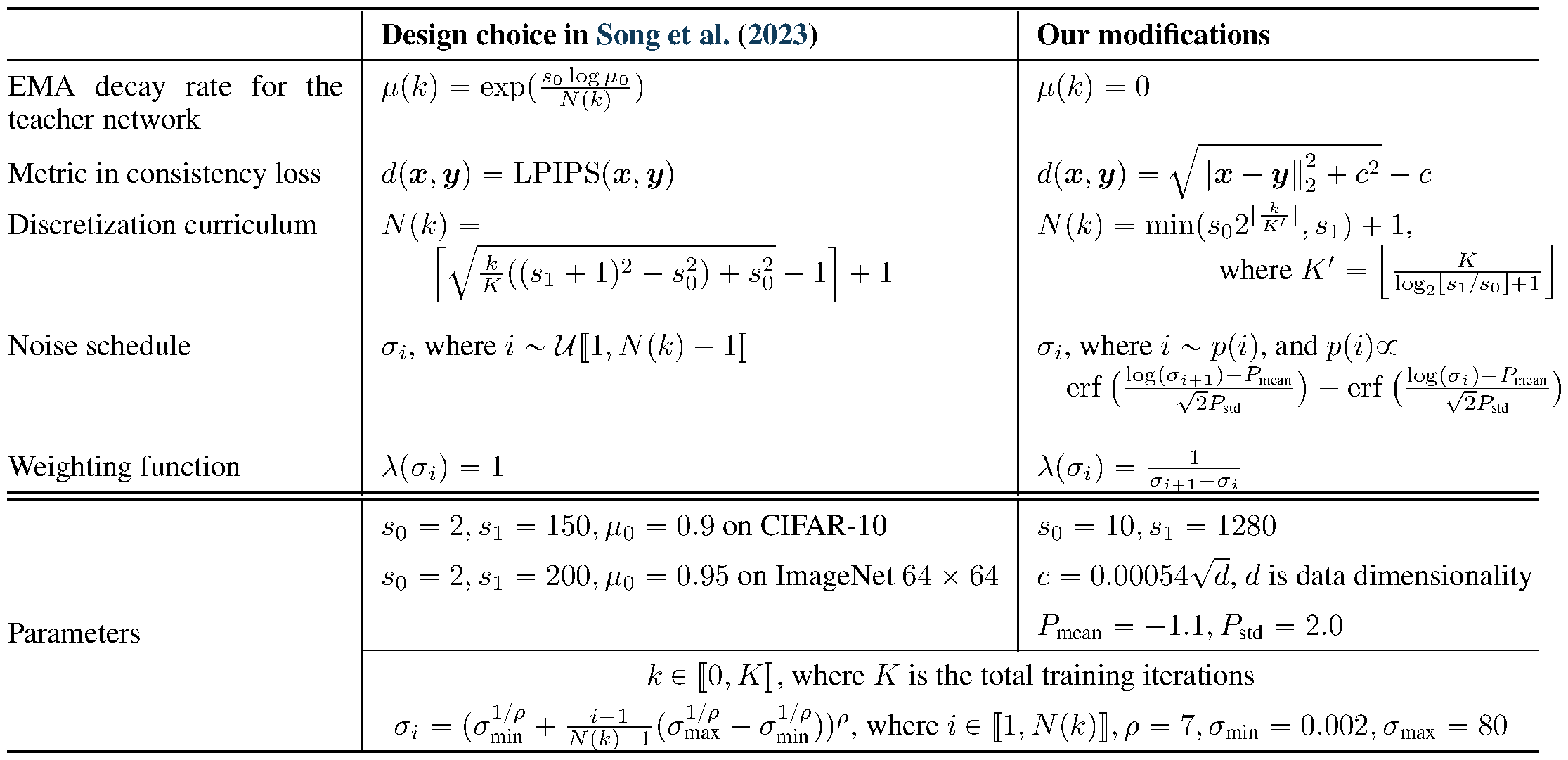
• No EMA on the teacher network (§3.2). Of the two arguments tying CT to consistency matching, the gradient one holds only when ${\theta }^{-}=\theta$; with an EMA teacher the $N\to \infty$ limit is not even a valid objective — a Dirac toy example breaks it. So $\mu =0$, on the teacher side only.

• Pseudo-Huber replaces LPIPS (§3.3). $d=\sqrt{\Vert x-y{\Vert }_2^2+c^2}-c$ with $c=0.00054\sqrt{d}$ sits between ${\ell }_2$ and ${\ell }_1$: it beats ${\ell }_2$ outright and catches LPIPS once $N(k)$ grows large — no feature network left to backpropagate through, and the heuristic scales $c$ with data dimensionality.

• Schedules and small knobs (§3.1, §3.4–3.5). $N(k)$ doubles from 10 up to 1280 across training; noise levels draw from a discretized lognormal ($P_{\mathrm{m}\mathrm{e}\mathrm{a}\mathrm{n}}=-1.1$, $P_{\mathrm{s}\mathrm{t}\mathrm{d}}=2$); weighting $\lambda =1/({\sigma }_{i+1}-{\sigma }_i)$; plus a smaller Fourier scale (0.02) and genuinely large dropout (0.3 on CIFAR-10).

• Experiments (§4, Tab. 2–3). CIFAR-10 and ImageNet-64 by FID, IS, precision and recall, GANs with pretrained discriminators excluded: iCT reads 2.83 / 2.46 at 1 / 2 steps on CIFAR-10 and 4.02 / 3.20 on ImageNet, iCT-deep 2.51 / 2.24 and 3.25 / 2.77 — past CD and TRACT.

• Recall, and thin margins (§4). ImageNet-64 recall rises to 0.63 from CT's 0.47 and BigGAN-deep's 0.48; one-step iCT edges StyleGAN-ADA on CIFAR-10 (2.83 vs 2.92) and BigGAN-deep on ImageNet (4.02 vs 4.06); two-step iCT-deep's 2.24 ties Score SDE's 2.20 at 2000 steps.

Consistency distillation moves into Stable Diffusion's latent space, swallows classifier-free guidance in one stage, and lands 768px in 2–4 steps.

• Latent consistency distillation (§4.1). The consistency function moves to SD's latent space, $f_{\theta }(z_t,c,t)\mapsto z_0$, parameterized on the teacher's own noise prediction and initialized from it; the ODE solver $\Psi$ — DDIM or DPM-Solver — appears only in training, never at inference.

• Guidance folded in, one stage (§4.2). The augmented ODE runs on the guided noise $(1+\omega ){ϵ}_c-\omega {ϵ}_{\varnothing }$ — its solver estimate is two solver calls combined — with the student conditioned on $\omega ~U[2,14]$. Guided-Distill took two stages and 45 A100-days; LCM, 32 A100-hours.

• Skipping-step (§4.3). Adjacent times on SD's 1000-step schedule sit so close that the consistency loss nearly vanishes and convergence crawls; aligning $t_{n+k}$ with $t_n$ at $k=20$ cuts the effective schedule from a thousand points to dozens; convergence lands in 2,000 iterations.

• Latent consistency fine-tuning (§4.4). A trained LCM adapts to custom image datasets without giving up its few-step inference.

• Experiments (§5). LAION-Aesthetics-6+ (12M, 512px) and 6.5+ (650K, 768px) from SD2.1, FID and CLIP on 30K images at $\omega =8$: 768px LCM reads 34.22 / 16.32 / 13.53 FID at 1 / 2 / 4 steps against Guided-Distill's 120.28 / 30.70 / 16.70 and DPM++'s 188.91 / 67.14 / 20.08.

• Guided-Distill was reproduced small (§5). Its numbers are a re-implementation at batch 72, 100K iterations, not the paper's batch 512 on 32 A100s — an admitted handicap: the claim is faster convergence at equal compute, no ceiling; $k=50$ suits DPM/DPM++, breaks DDIM.

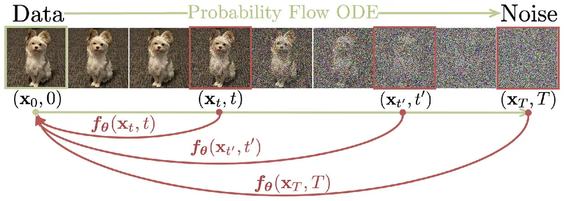
One evaluation maps noise straight to data — learn the map from any ODE point to its origin, distilled from a teacher or trained from scratch.

• The consistency function (§3, Fig. 1). $f(x_t,t)\mapsto x_{ϵ}$ sends every point of the probability-flow ODE to its origin, so sampling is a single network evaluation at $x_T$; self-consistency — every point of one trajectory shares an output — is the property both training modes below enforce.

• The boundary condition (§3, Eq. 5). $f(·,ϵ)$ must be the identity, or $f\equiv 0$ solves everything; it comes almost for free from the skip form $c_{\mathrm{s}\mathrm{k}\mathrm{i}\mathrm{p}}(t)x+c_{\mathrm{o}\mathrm{u}\mathrm{t}}(t)F_{\theta }(x,t)$ with $c_{\mathrm{s}\mathrm{k}\mathrm{i}\mathrm{p}}(ϵ)=1$, $c_{\mathrm{o}\mathrm{u}\mathrm{t}}(ϵ)=0$ — the EDM-style shape that lets existing diffusion architectures drop in unchanged.

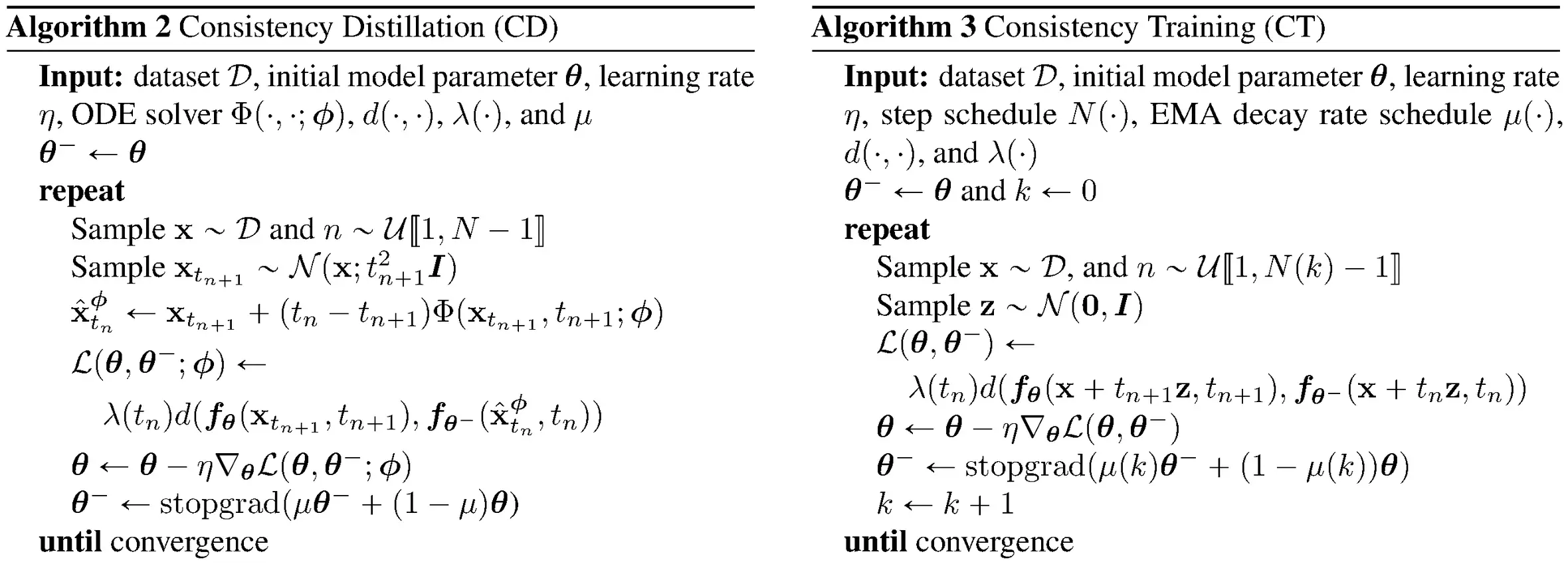
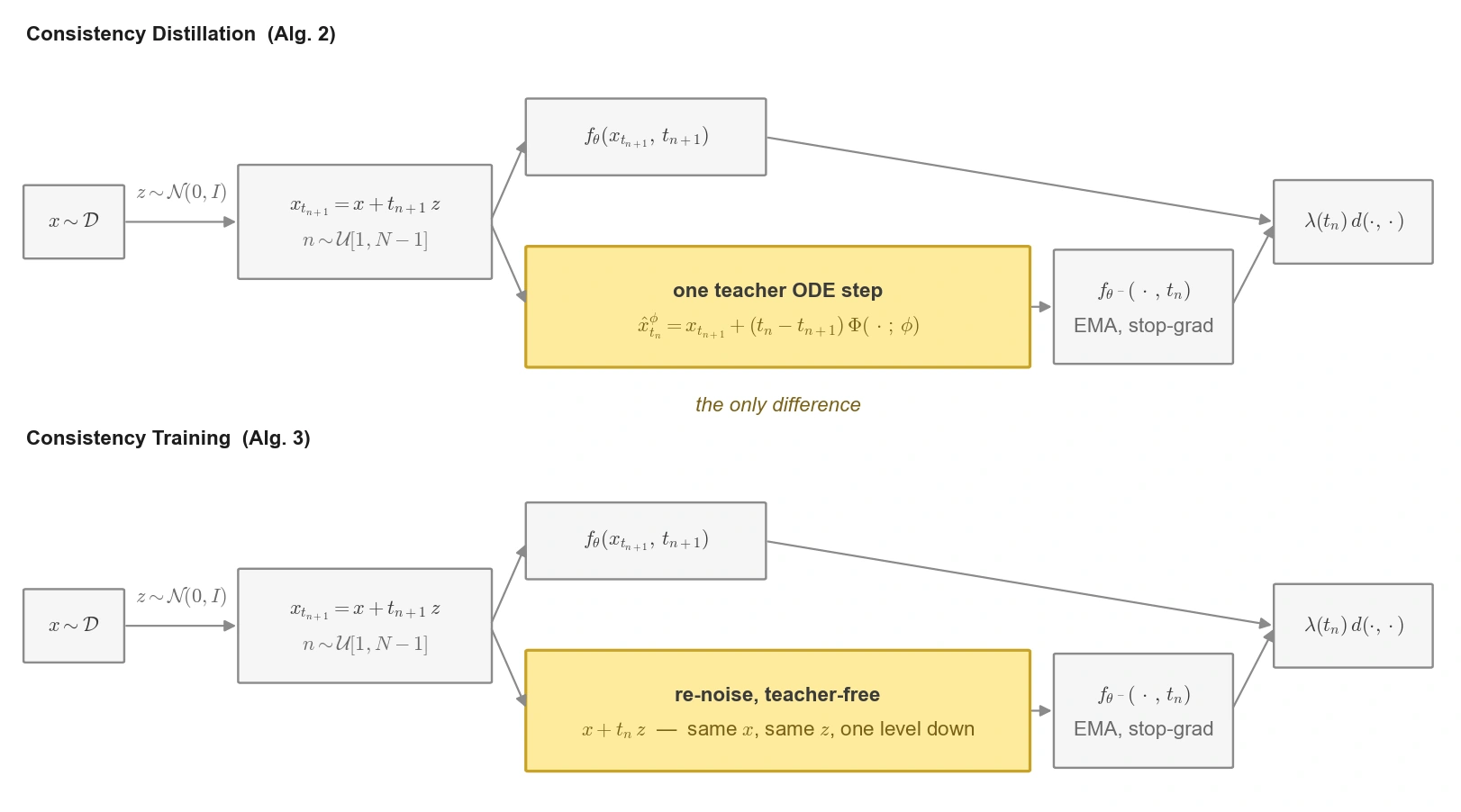
• Consistency distillation (§4, Alg. 2). Noise an image to $x_{t_{n+1}}$, take one teacher step back, and pull the two outputs together — the target side from an EMA copy, stopgradded. With LPIPS and $N=18$: CIFAR-10 3.55, ImageNet-64 6.20 one-step, past PD everywhere but one point.

• Consistency training (§5, Alg. 3). Swap the teacher's score for the unbiased estimate $-(x_t-x)/t^2$: the pair becomes $x+t_{n}z$ and $x+t_{n+1}z$ with one shared $z$, no diffusion model anywhere — a standalone family that still matches PD's one step, with $N$ and $\mu$ grown on schedules.

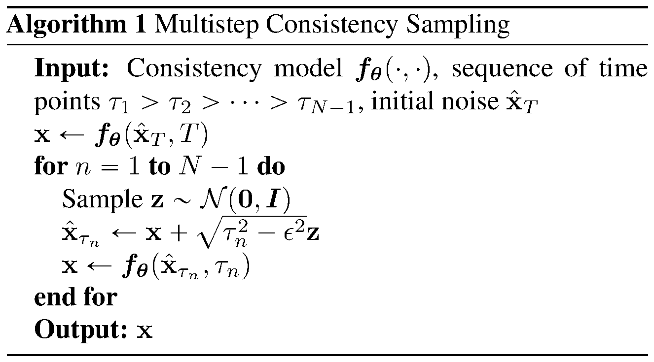
• Multistep sampling (Alg. 1). Alternate the model with re-noising to a lower level, time points picked greedily by ternary search; extra compute buys quality back, and mapping any $x_t$ to $x_{ϵ}$ gives zero-shot inpainting, colorization, super-resolution and stroke-guided editing.

• Experiments (§6). CIFAR-10, ImageNet-64, LSUN Bedroom / Cat by FID, IS, precision, recall, from EDM teachers: CD beats PD at 1–2 steps everywhere but one point and the synthetic-data distillers; CT, teacher-free, gets 8.70 / 5.83 on CIFAR-10, past every VAE and flow.

• The metric is half the margin (§6.2). PD retrained with LPIPS improves uniformly on its ${\ell }_2$ (Fig. 4), so part of CD's lead is the metric, not the objective; Heun and $N=18$ come from EDM unchanged, and CT samples share structure with EDM's from one noise — no mode collapse.

Both trainers in one routine, straight from the repo, cut to the lines that carry the idea:

# The parameterization (karras_diffusion.py, denoise): f(x, s_min) = x by construction.
c_skip = sd**2 / ((sigma - s_min)**2 + sd**2)  # EDM's scalings with sigma -> sigma - s_min
c_out = (sigma - s_min) * sd / (sigma**2 + sd**2)**0.5  # at s_min: c_skip = 1, c_out = 0
f = c_skip * x_t + c_out * unet(c_in * x_t, 250 * log(sigma))  # nothing left to learn there

# One routine serves both modes (consistency_losses): adjacent Karras levels t > t2.
x_t = x + t * z  # noise a real image
pred = f(x_t, t, theta)  # the trainable side; dropout RNG state saved here
with no_grad():  # one solver step t -> t2 builds the trajectory pair
    denoiser = teacher_denoise(x_t, t) if distill else x  # CT: the raw image is the score
    d = (x_t - denoiser) / t  # CD upgrades this to Heun with a second evaluation at t2
    x_t2 = x_t + (t2 - t) * d
    target = f(x_t2, t2, theta_ema).detach()  # EMA copy, rerun under the student's dropout mask
loss = lpips(pred, target)  # or plain l2; LPIPS inputs are resized up to 224px first

# Sampling is f(s_max * z, s_max); Alg. 1 re-noises lower and applies f again for quality.